A first example: exponential growth
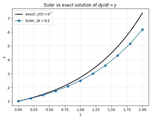
Take the most famous ODE of all: In words: the rate of change of equals itself. Populations, compound interest, and unstable physical systems all obey this law in some regime. You can write down the closed-form solution by inspection: the only function whose derivative equals itself is the exponential, so That is the analytical solution. For most ODEs you encounter in practice there is no analytical solution, and you have to compute numerically. The simplest numerical method is the Euler method.The Euler method
The idea is to take a tiny step in the direction the derivative tells you to go, then repeat. Pick a small step size . Starting from , replace the smooth ODE with a discrete update: At each step you compute the slope at the current point and take a step of length in that direction. After steps you have an approximation of at time . Two lines of Python implement it.Show plotting code
Show plotting code
- What happens if you shrink ?
- How fast does the error shrink as ?
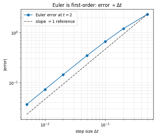
Step size and error
The Euler method is first-order accurate: the global error at a fixed final time scales linearly with . Halving roughly halves the error. You can verify this by running Euler at several step sizes and plotting the error at on a log-log axis. A first-order method gives a straight line of slope 1.Show plotting code
Show plotting code
A 2D example: rotation
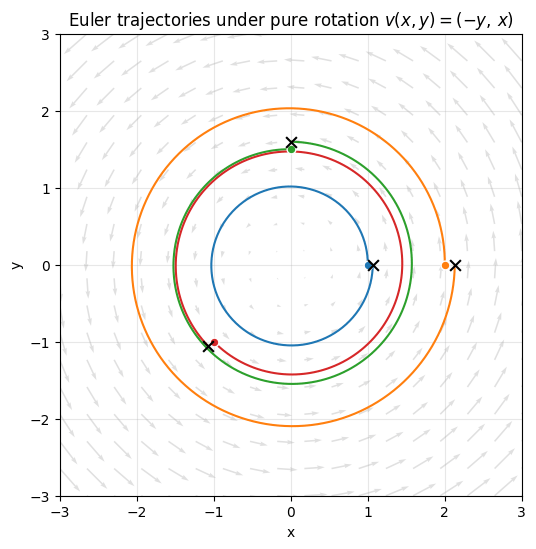
ODEs are not restricted to scalar . The state can be a vector , and the right-hand side becomes a vector-valued function : The vector field assigns a velocity to every point in space, and the ODE says follow that velocity. The Euler update is identical, just vectorized: A clean 2D example is pure rotation: Each particle at position gets a velocity perpendicular to its position vector. The exact trajectories are circles around the origin, traced counterclockwise.Show plotting code
Show plotting code
Where this leads
That last figure is the whole picture of how modern generative models sample. Replace the hand-written rotation field with a learned vector field , parameterized by a neural network. Start the particles from Gaussian noise instead of arbitrary points. Run the same Euler loop you just wrote.- If was trained to match a target velocity field connecting Gaussian noise to the data distribution, you have flow matching.
- If encodes the score of a noise-perturbed data distribution, you have a diffusion model in its probability-flow ODE form.
References
- L. C. Evans, Partial Differential Equations (Chapter 1), for ODE basics and existence/uniqueness.
- E. Hairer, S. P. Nørsett, G. Wanner, Solving Ordinary Differential Equations I, the standard reference on Euler and its successors.
- Khan Academy, Differential equations, for a gentler video-first introduction.