EKF Localization

The Markov localization section applies the Bayes filter to a robot with a known map, and contrasts global localization, where the initial pose is unknown, with tracking, where it is approximately known. This section treats the tracking case with a Gaussian belief, first in one dimension and then for a ground robot with the extended Kalman filter.

Tracking

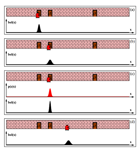
Just like localization, tracking can refer to location prediction of the agent itself or the objects that the agents perceives in its environment. For tracking we are given the initial pose

s_0

that is approximately known. It is common to initialize the belief with a narrow Gaussian distribution around

\hat{s}_0

\mathtt{bel}(s_0) = \mathcal{N}(s_0-\hat s_0, \Sigma)

Lets look at a similar example to the localization problem:

Example environment for tracking - a hallway with three identical and labeled doors The original belief is a normal distribution centered around door 1 where the agent is initially placed. As the robot moves to the right, its belief is convolved with the Gaussian transition / motion model. The resulting belief is a shifted Gaussian of increased width. Now suppose the robot detects that it is in front of door 2. Folding this measurement probability into the robot’s belief yields the posterior shown in (c). Note that the variance of the resulting belief is smaller than the variances of both the robot’s previous belief and the observation density. This is natural, since integrating two independent estimates should make the robot more certain than each estimate in isolation. After moving down the hallway, the robot’s uncertainty in its position increases again, since the tracker continues to incorporate motion uncertainty into the robot’s belief.

EKF localization with known correspondences

The hallway examples use a one-dimensional state. A ground robot such as the TurtleBot has the pose

s_t = (x, y, \theta)

, and the extended Kalman filter tracks a Gaussian belief over it. Like the tracking example above, EKF localization needs a good initial guess: the belief is a single Gaussian, so it cannot represent the multimodal beliefs of global localization. The map

m

is a set of point landmarks with known positions

m_j = (m_{j,x}, m_{j,y})

. At each step the robot measures the range

r^i_t

and the bearing

\phi^i_t

to every landmark it can see,

z^i_t = (r^i_t, \phi^i_t)

. Known correspondences means that it also knows which landmark produced each measurement: the correspondence variable

c^i_t = j

names the landmark. A robot gets this for free when every landmark carries a unique code, such as a fiducial marker whose ID the camera reads.

Motion model

The action is the pair of wheel speeds

a_t = (u_L, u_R)

. As in the EKF section, they set the forward speed

v = \frac{r}{2}(u_L + u_R)

and the turning rate

\omega = \frac{r}{2d}(u_R - u_L)

. Holding

v

and

\omega

constant for

\Delta t

moves the robot along an arc of radius

v/\omega

g(a_t, s_{t-1}) = \begin{bmatrix} x - \frac{v}{\omega}\sin\theta + \frac{v}{\omega}\sin(\theta + \omega\Delta t) \\ y + \frac{v}{\omega}\cos\theta - \frac{v}{\omega}\cos(\theta + \omega\Delta t) \\ \theta + \omega\Delta t \end{bmatrix}.

Its Jacobian with respect to the state is

G_t = \begin{bmatrix} 1 & 0 & \frac{v}{\omega}\left(\cos(\theta + \omega\Delta t) - \cos\theta\right) \\ 0 & 1 & \frac{v}{\omega}\left(\sin(\theta + \omega\Delta t) - \sin\theta\right) \\ 0 & 0 & 1 \end{bmatrix},

evaluated at

\mu_{t-1}

. The noise comes from the wheels. Each wheel turns at its commanded speed plus Gaussian noise, with covariance

M_t

in wheel-speed space. The Jacobian

V_t = \partial g / \partial a_t

maps that noise into the state, so the motion noise covariance is

R_t = V_t M_t V_t^\top

Measurement model

For landmark

j

, write

\delta = (m_{j,x} - x,\; m_{j,y} - y)

and

q = \delta^\top\delta

. The predicted measurement and its Jacobian are

h(s_t, j, m) = \begin{bmatrix} \sqrt{q} \\ \operatorname{atan2}(\delta_y, \delta_x) - \theta \end{bmatrix}, \qquad H^i_t = \frac{1}{q}\begin{bmatrix} -\sqrt{q}\,\delta_x & -\sqrt{q}\,\delta_y & 0 \\ \delta_y & -\delta_x & -q \end{bmatrix},

evaluated at the predicted mean

\bar\mu_t

, with measurement noise covariance

Q_t = \operatorname{diag}(\sigma_r^2, \sigma_\phi^2)

The algorithm

One step takes the previous belief, the action, the measurements and their correspondences, and the map:

\begin{array}{ll} 1: & \bar\mu_t = g(a_t, \mu_{t-1}) \\ 2: & \bar\Sigma_t = G_t\, \Sigma_{t-1}\, G_t^\top + V_t M_t V_t^\top \\ 3: & \text{for each observed feature } z^i_t \text{ with } j = c^i_t: \\ 4: & \qquad \hat z^i_t = h(\bar\mu_t, j, m), \quad \text{and } H^i_t \text{ at } \bar\mu_t \\ 5: & \qquad K^i_t = \bar\Sigma_t H^{i\top}_t \left(H^i_t \bar\Sigma_t H^{i\top}_t + Q_t\right)^{-1} \\ 6: & \qquad \bar\mu_t \leftarrow \bar\mu_t + K^i_t \left(z^i_t - \hat z^i_t\right) \\ 7: & \qquad \bar\Sigma_t \leftarrow \left(I - K^i_t H^i_t\right) \bar\Sigma_t \\ 8: & \mu_t = \bar\mu_t, \quad \Sigma_t = \bar\Sigma_t \end{array}

The loop folds in one landmark at a time. Each update starts from the belief left by the previous one, which is exact for a linear-Gaussian model when the measurement noises are independent. The bearing residual in line 6 is wrapped to

(-\pi, \pi]

, since an angle error of

2\pi - 0.01

is really

-0.01

. This algorithm follows the EKF localization algorithm in Chapter 7 of Probabilistic Robotics (Thrun, Burgard and Fox), with

s

for the state,

a

for the action, and wheel speeds for the action.

%config InlineBackend.figure_formats = ["svg"]

import matplotlib.pyplot as plt
import numpy as np
from cycler import cycler

plt.rcParams.update(
    {
        "figure.figsize": (6.5, 3.5),  # matches the 6.5 in text column
        "font.size": 9,
        "axes.titlesize": 10,
        "axes.labelsize": 9,
        "xtick.labelsize": 8,
        "ytick.labelsize": 8,
        "legend.fontsize": 8,
        "axes.prop_cycle": cycler(
            color=["#0072B2", "#D55E00", "#009E73", "#cb77a6", "#c28600", "#1d99e0", "#7f7f7f"]
        ),
        "axes.grid": True,
        "grid.alpha": 0.3,
        "svg.fonttype": "path",
    }
)

# named colors from the palette above
BLUE, VERMILLION, GREEN, PINK, GOLD, SKY, GRAY = (
    "#0072B2", "#D55E00", "#009E73", "#cb77a6", "#c28600", "#1d99e0", "#7f7f7f",
)

np.random.seed(7)

r, d = 0.033, 0.1435  # TurtleBot3 Waffle wheel radius and half wheel separation, in meters
dt = 0.5  # seconds per step


def wrap(angle):
    """Wrap an angle to (-pi, pi]."""
    return (angle + np.pi) % (2 * np.pi) - np.pi


def twist(a):
    """Forward speed v and turning rate w from the wheel speeds a = (u_L, u_R)."""
    u_L, u_R = a
    return r / 2 * (u_L + u_R), r / (2 * d) * (u_R - u_L)


def g(a, s, dt=dt):
    """Velocity motion model: the pose after holding the wheel speeds a for dt.

    s is one pose (x, y, theta) or an array of shape (3, n) of poses.
    """
    v, w = twist(a)
    x, y, th = s
    if abs(w) < 1e-9:  # straight line, the limit of the arc
        return np.array([x + v * dt * np.cos(th), y + v * dt * np.sin(th), th])
    return np.array([
        x - v / w * np.sin(th) + v / w * np.sin(th + w * dt),
        y + v / w * np.cos(th) - v / w * np.cos(th + w * dt),
        wrap(th + w * dt),
    ])


def G(a, s, dt=dt):
    """Jacobian of g with respect to the state."""
    v, w = twist(a)
    th = s[2]
    if abs(w) < 1e-9:
        return np.array([[1, 0, -v * dt * np.sin(th)], [0, 1, v * dt * np.cos(th)], [0, 0, 1]])
    return np.array([
        [1, 0, v / w * (np.cos(th + w * dt) - np.cos(th))],
        [0, 1, v / w * (np.sin(th + w * dt) - np.sin(th))],
        [0, 0, 1],
    ])


def V(a, s, dt=dt):
    """Jacobian of g with respect to the wheel speeds (u_L, u_R)."""
    v, w = twist(a)
    th = s[2]
    s0, c0, s1, c1 = np.sin(th), np.cos(th), np.sin(th + w * dt), np.cos(th + w * dt)
    if abs(w) < 1e-9:  # straight line: the limit of the arc derivatives
        dg_dvw = np.array([[c0 * dt, -v * s0 * dt**2 / 2], [s0 * dt, v * c0 * dt**2 / 2], [0, dt]])
        return dg_dvw @ np.array([[r / 2, r / 2], [-r / (2 * d), r / (2 * d)]])
    dg_dvw = np.array([
        [(s1 - s0) / w, v * (s0 - s1) / w**2 + v * c1 * dt / w],
        [(c0 - c1) / w, -v * (c0 - c1) / w**2 + v * s1 * dt / w],
        [0, dt],
    ])
    dvw_du = np.array([[r / 2, r / 2], [-r / (2 * d), r / (2 * d)]])
    return dg_dvw @ dvw_du


def h(s, j, m):
    """Range and bearing from the pose s to landmark j of the map m."""
    dx, dy = m[j] - s[:2]
    return np.array([np.hypot(dx, dy), wrap(np.arctan2(dy, dx) - s[2])])


def H(s, j, m):
    """Jacobian of h with respect to the state."""
    dx, dy = m[j] - s[:2]
    q = dx**2 + dy**2
    sq = np.sqrt(q)
    return np.array([[-sq * dx, -sq * dy, 0], [dy, -dx, -q]]) / q

def ekf_localization(mu, Sigma, a, z, c, m, M, Q, dt=dt):
    """One step of EKF localization with known correspondences.

    z holds one (range, bearing) row per observed landmark and c the landmark index of each row.
    """
    G_t, V_t = G(a, mu, dt), V(a, mu, dt)
    mu_bar = g(a, mu, dt)  # line 1
    Sigma_bar = G_t @ Sigma @ G_t.T + V_t @ M @ V_t.T  # line 2
    for z_i, j in zip(z, c):  # line 3
        z_hat, H_i = h(mu_bar, j, m), H(mu_bar, j, m)  # line 4
        K_i = Sigma_bar @ H_i.T @ np.linalg.inv(H_i @ Sigma_bar @ H_i.T + Q)  # line 5
        innovation = z_i - z_hat
        innovation[1] = wrap(innovation[1])
        mu_bar = mu_bar + K_i @ innovation  # line 6
        mu_bar[2] = wrap(mu_bar[2])
        Sigma_bar = (np.eye(3) - K_i @ H_i) @ Sigma_bar  # line 7
    return mu_bar, Sigma_bar  # line 8

One step with one landmark

Start with a single step, the setting of the EKF section. The robot drives straight down the page, at heading

\theta = -90°

, at 0.25 m/s for 4 s. Its belief knows the starting position to 2 cm but the heading only to

30°

, and the motion noise is left out to isolate the heading. A single landmark,

m_1 = (0, -2)

m, stands straight ahead. The robot’s true heading during the drive was

25°

off the nominal one, so it really stopped at about

(0.42, -0.91)

m. From there its sensor measures the range and bearing to

m_1

, with noise

\sigma_r = 5

cm and

\sigma_\phi = 2°

. The code runs one step of ekf_localization. For comparison it also computes the exact posterior: it pushes samples of the starting pose through

g

, weights each one by the likelihood of the measurement, and resamples.

sigma_r, sigma_phi = 0.05, np.deg2rad(2)  # range and bearing noise
Q = np.diag([sigma_r**2, sigma_phi**2])

u = 0.25 / r
a_straight = np.array([u, u])  # equal wheel speeds: straight ahead at 0.25 m/s
m_one = np.array([[0.0, -2.0]])
mu0 = np.array([0.0, 0.0, -np.pi / 2])
Sigma0 = np.diag([0.02**2, 0.02**2, np.deg2rad(30) ** 2])
no_noise = np.zeros((2, 2))

# the true pose and the measurement taken from it
s_true1 = g(a_straight, mu0 + np.array([0, 0, np.deg2rad(25)]), dt=4.0)
z1 = h(s_true1, 0, m_one) + np.random.normal(0, [sigma_r, sigma_phi])

# EKF: prediction alone, then the full step with the measurement
mu_pred, Sigma_pred = ekf_localization(mu0, Sigma0, a_straight, [], [], m_one, no_noise, Q, dt=4.0)
mu1, Sigma1 = ekf_localization(mu0, Sigma0, a_straight, [z1], [0], m_one, no_noise, Q, dt=4.0)

# exact posterior: push samples through g, weight them by the measurement likelihood, resample
n_samples = 100_000
pred = g(a_straight, np.random.multivariate_normal(mu0, Sigma0, n_samples).T, dt=4.0)
dx, dy = m_one[0, 0] - pred[0], m_one[0, 1] - pred[1]
res_r = z1[0] - np.hypot(dx, dy)
res_phi = wrap(z1[1] - wrap(np.arctan2(dy, dx) - pred[2]))
w = np.exp(-(res_r**2) / (2 * sigma_r**2) - res_phi**2 / (2 * sigma_phi**2))
post = pred[:, np.random.choice(n_samples, size=n_samples, p=w / w.sum())]

print("measured range, bearing:", z1.round(3), " predicted:", h(mu_pred, 0, m_one).round(3))
print("true          x, y:", s_true1[:2].round(3))
print("EKF predicted x, y:", mu_pred[:2].round(3), "std:", np.sqrt(np.diag(Sigma_pred)[:2]).round(3))
print("EKF updated   x, y:", mu1[:2].round(3), "std:", np.sqrt(np.diag(Sigma1)[:2]).round(3))
print("exact post.   x, y:", post[:2].mean(axis=1).round(3), "std:", post[:2].std(axis=1).round(3))

measured range, bearing: [ 1.257 -0.821]  predicted: [1. 0.]
true          x, y: [ 0.423 -0.906]
EKF predicted x, y: [ 0. -1.] std: [0.524 0.02 ]
EKF updated   x, y: [ 0.41  -0.965] std: [0.02  0.019]
exact post.   x, y: [ 0.441 -0.887] std: [0.022 0.022]

The predicted samples form the banana from the EKF section, opening upward because the robot drives down the page. The EKF’s prediction ellipse is wide in

x

, where a heading error moves the robot sideways. In

y

, the direction of travel, it is only 2 cm tall, because the Jacobian passes no heading uncertainty into the forward position. The two parts of the measurement do different jobs. The bearing,

-0.82

rad or about

-47°

, puts the landmark well to the robot’s right. Only samples on the right arm of the banana agree with that, so the bearing removes the left-right ambiguity that a range alone would leave. The EKF uses it too. At the predicted mean the bearing row of

H_t

couples

x

and

\theta

, and the update moves the mean to

x = 0.41

m, close to the true 0.42 m, with 2 cm of uncertainty. The range, 1.257 m against a predicted 1.0 m, says the robot stopped short. Here the EKF falls short. Its predicted

y

uncertainty was only 2 cm, so it moves

y

only from

-1.0

-0.965

m, and the true

y = -0.906

m ends up about three of its standard deviations away. The exact posterior, centered at

(0.44, -0.89)

m, has no such problem. This is the overconfidence from the EKF section, now inside a localization step.

Driving among landmarks

Over many steps, the code below drives a simulated TurtleBot3 Waffle around a circle of radius 1.5 m at 0.2 m/s for 70 s, about one and a half laps. Three landmarks stand outside the circle. The range-bearing sensor sees a landmark only within 1.5 m, so on parts of the circle no landmark is visible. Each wheel of the simulated robot turns at its commanded speed plus noise, with a standard deviation of 5% of the speed plus 0.1 rad/s. The filter knows this noise model, which gives it

M_t

. The sensor noise is the same as in the single step. The filter starts from the true pose with a small uncertainty. For comparison, the same filter also runs without any measurements, which is dead reckoning from the wheel speeds alone.

# map: three landmarks outside the circle
m = 2.5 * np.array([[np.cos(t), np.sin(t)] for t in np.deg2rad([0, 120, 240])])
max_range = 1.5

# commanded wheel speeds for a counterclockwise circle of radius 1.5 m at 0.2 m/s
v_cmd, w_cmd = 0.2, 0.2 / 1.5
a_cmd = np.array([(v_cmd - d * w_cmd) / r, (v_cmd + d * w_cmd) / r])
sigma_u = 0.05 * np.abs(a_cmd) + 0.1
M = np.diag(sigma_u**2)

n_steps = 140
s = np.array([1.5, 0.0, np.pi / 2])  # true start pose
mu, Sigma = s.copy(), np.diag([0.05**2, 0.05**2, np.deg2rad(5) ** 2])
mu_dr, Sigma_dr = mu.copy(), Sigma.copy()

true_path, ekf_path, ekf_cov, dr_path, dr_cov, n_seen = [s], [mu], [Sigma], [mu_dr], [Sigma_dr], [0]
for t in range(n_steps):
    s = g(a_cmd + np.random.normal(0, sigma_u), s)  # the robot moves with noisy wheels
    z, c = [], []
    for j in range(len(m)):  # sense every landmark in range
        z_true = h(s, j, m)
        if z_true[0] <= max_range:
            z.append(z_true + np.random.normal(0, [sigma_r, sigma_phi]))
            c.append(j)
    mu, Sigma = ekf_localization(mu, Sigma, a_cmd, z, c, m, M, Q)
    mu_dr, Sigma_dr = ekf_localization(mu_dr, Sigma_dr, a_cmd, [], [], m, M, Q)
    true_path.append(s); ekf_path.append(mu); ekf_cov.append(Sigma)
    dr_path.append(mu_dr); dr_cov.append(Sigma_dr); n_seen.append(len(c))

true_path, ekf_path, dr_path = map(np.array, (true_path, ekf_path, dr_path))
ekf_cov, dr_cov, n_seen = np.array(ekf_cov), np.array(dr_cov), np.array(n_seen)
err = ekf_path - true_path
err[:, 2] = wrap(err[:, 2])
inside = np.abs(err) <= 2 * np.sqrt(ekf_cov[:, [0, 1, 2], [0, 1, 2]])
print(f"steps with a landmark in view: {np.mean(n_seen > 0):.0%}")
print("final position error, EKF:", np.round(np.hypot(*err[-1, :2]), 3), "m",
      " dead reckoning:", np.round(np.hypot(*(dr_path[-1, :2] - true_path[-1, :2])), 3), "m")
print("fraction of steps inside 2 sigma (x, y, theta):", inside.mean(axis=0).round(2))

steps with a landmark in view: 55%
final position error, EKF: 0.092 m  dead reckoning: 0.352 m
fraction of steps inside 2 sigma (x, y, theta): [0.99 0.99 0.98]

The first figure shows the paths and every tenth

2\sigma

ellipse of the EKF. Without measurements the estimate drifts: after 70 s dead reckoning is 35 cm from the true position, against 9 cm for the EKF. The EKF ellipses grow while no landmark is in view and shrink again as soon as one comes into range, the same pattern as the hallway tracking example, now in two dimensions with heading. The second figure checks whether the filter is honest about its uncertainty. A consistent filter keeps its error inside the

\pm 2\sigma

band about 95% of the time. The band widens in the gray stretches with no landmark in view and narrows when a landmark appears. Here the robot drives on gentle arcs and its heading uncertainty stays small, so linearization works well: the error stays inside the band at 98 to 99% of the steps. With a wide heading belief the same filter can become overconfident, as the EKF section shows. Key references: (Sabinasz, 2017; Li et al., 2018; Khan et al., 2004; Hofmann et al., 2013; Peršić et al., 2019)

References

Hofmann, M., Wolf, D., Rigoll, G. (2013). Hypergraphs for Joint Multi-view Reconstruction and Multi-object Tracking. 2013 IEEE Conference on Computer Vision and Pattern Recognition.
Khan, Z., Balch, T., Dellaert, F. (2004). A Rao-Blackwellized particle filter for EigenTracking. Proceedings of the 2004 IEEE Computer Society Conference on Computer Vision and Pattern Recognition, 2004. CVPR 2004.
Li, X., Ylioinas, J., Kannala, J. (2018). Full-Frame Scene Coordinate Regression for Image-Based Localization. arXiv [cs.CV].
Peršić, J., Petrović, L., Marković, I., Petrović, I. (2019). Spatio-Temporal Multisensor Calibration Based on Gaussian Processes Moving Object Tracking. arXiv [cs.RO].
Sabinasz, D. (2017). Robot Localization II: The Histogram Filter.

Found an error on this page? Report an issue.

State Estimation & Mapping

State Estimation

SLAM

Tracking

EKF localization with known correspondences

Motion model

Measurement model

The algorithm

One step with one landmark

Driving among landmarks

References

​Tracking

​EKF localization with known correspondences

​Motion model

​Measurement model

​The algorithm

​One step with one landmark

​Driving among landmarks

​References

Tracking

EKF localization with known correspondences

Motion model

Measurement model

The algorithm

One step with one landmark

Driving among landmarks

References