Nonholonomic Wheeled Robots

A nonholonomic robot has conventional wheels that cannot slide sideways. The wheeled robots overview introduces the wheel types, the chassis configuration

q = (\theta, x, y)

and the body twist

\mathcal{V}_b

used below. You will derive the kinematic model of a differential-drive robot, test its no-slip assumption on a grippy floor and on ice, and use the model for wheel odometry. This section follows chapter 13, Wheeled Mobile Robots, of Kevin Lynch and Frank Park, Modern Robotics: Mechanics, Planning, and Control (Cambridge University Press, 2017) (Kevin M. Lynch, 2017).

import math
from pathlib import Path

import matplotlib.pyplot as plt
import numpy as np
import rerun as rr
import rerun.blueprint as rrb
import warp as wp

wp.config.log_level = wp.LOG_WARNING
import newton
import newton.viewer

RECORDINGS = Path("recordings")
RECORDINGS.mkdir(exist_ok=True)

Simulating the robot

The simulations use Newton, a physics engine for robotics built on NVIDIA Warp (Data Curation for Machine Lear, n.d.). The robot consists of rigid links connected by joints. Its collision shapes have a friction coefficient

\mu

. Each wheel is a link on a revolute joint. Its motor tracks a commanded angular speed. The floor is a plane. The simulation has no built-in knowledge of

H(0)

or the no-slip condition. The chassis moves because friction at each contact pushes on the wheels. The helpers below run a simulation at 60 frames per second. They command the wheel speeds at each frame and record the chassis pose

(\theta, x, y)

and the wheel angles. The body twist is measured from the recorded poses using the definition above. You can also record each run for the Rerun viewer. It draws the robot, paths and signals on a timeline that you can scrub.

def planar_pose(body_q):
    # (theta, x, y) of a body from its Newton transform (px, py, pz, qx, qy, qz, qw)
    px, py, _, qx, qy, qz, qw = body_q
    theta = math.atan2(2 * (qw * qz + qx * qy), 1 - 2 * (qy * qy + qz * qz))
    return theta, px, py


def measured_body_twist(t, pose):
    # finite-difference the pose, then map q_dot to V_b = (omega_bz, v_bx, v_by)
    theta = np.unwrap(pose[:, 0])
    th_dot, x_dot, y_dot = (np.gradient(v, t) for v in (theta, pose[:, 1], pose[:, 2]))
    c, s = np.cos(theta), np.sin(theta)
    return np.stack([th_dot, c * x_dot + s * y_dot, -s * x_dot + c * y_dot], axis=1)


def simulate(model, chassis, drives, wheel_speeds, duration, recording=None, on_frame=None, blueprint=None,
             fps=60, substeps=6):
    solver = newton.solvers.SolverMuJoCo(
        model, use_mujoco_contacts=False, disable_sensors=True, solver="newton", integrator="implicitfast",
        cone="elliptic", iterations=20, ls_iterations=50, njmax=2048, nconmax=1024,
    )
    state, next_state, control = model.state(), model.state(), model.control()
    newton.eval_fk(model, model.joint_q, model.joint_qd, state)
    collision = newton.CollisionPipeline(model, rigid_contact_max=1024)
    contacts = collision.contacts()
    drive_dofs = [int(model.joint_qd_start.numpy()[j]) for j in drives]
    drive_coords = [int(model.joint_q_start.numpy()[j]) for j in drives]
    target = control.joint_target_qd.numpy()
    dt = 1.0 / fps / substeps

    def advance():
        nonlocal state, next_state
        for _ in range(substeps):
            state.clear_forces()
            collision.collide(state, contacts)
            solver.step(state, next_state, control, contacts, dt)
            state, next_state = next_state, state

    graph = None
    if wp.get_device().is_cuda:
        with wp.ScopedCapture() as capture:
            advance()
        graph = capture.graph

    viewer = None
    if recording is not None:
        viewer = newton.viewer.ViewerRerun(app_id="wheeled_robots_" + recording.stem.split("-0")[0].replace("-", "_"),
                                           record_to_rrd=str(recording), keep_historical_data=True)
        viewer.set_model(model)
        if blueprint is not None:
            rr.send_blueprint(blueprint)

    t, times, poses, angles = 0.0, [], [], []
    for _ in range(int(duration * fps)):
        target[drive_dofs] = wheel_speeds(t)
        control.joint_target_qd.assign(target)
        wp.capture_launch(graph) if graph else advance()
        t += 1.0 / fps
        times.append(t)
        poses.append(planar_pose(state.body_q.numpy()[chassis]))
        angles.append(state.joint_q.numpy()[drive_coords])
        if viewer is not None:
            viewer.begin_frame(t)
            viewer.log_state(state)
            if on_frame is not None:
                on_frame(np.array(times), np.array(poses), np.array(angles))
            viewer.end_frame()
    if viewer is not None:
        viewer.close()
    return np.array(times), np.array(poses), np.array(angles)


def displace(q, twist, dt):
    # move the chassis at a constant body twist for time dt (exponential of the planar twist)
    w, vx, vy = np.asarray(twist) * dt
    if abs(w) < 1e-12:
        db = np.array([0.0, vx, vy])
    else:
        db = np.array([w, (vx * np.sin(w) + vy * (np.cos(w) - 1)) / w, (vy * np.sin(w) + vx * (1 - np.cos(w))) / w])
    c, s = np.cos(q[0]), np.sin(q[0])
    return q + np.array([db[0], c * db[1] - s * db[2], s * db[1] + c * db[2]])


def integrate_twists(q0, twists, dt):
    path = [np.asarray(q0, float)]
    for tw in twists[1:]:
        path.append(displace(path[-1], tw, dt))
    return np.array(path)


VIEWER = "https://artifacts.aegeanai.com/rerun/viewer/0.41.0/index.html?url="
RECORDING_URL = "https://artifacts.aegeanai.com/rerun/wheeled-robots/{}-0.41.rrd"


def show_recording(name, height=560):
    # the published recording in the self-hosted Rerun web viewer
    from urllib.parse import quote
    from IPython.display import IFrame
    src = VIEWER + quote(RECORDING_URL.format(name), safe="")
    return IFrame(src, width="100%", height=height, extras=['allow="fullscreen"', 'loading="lazy"'])


def path_strip(poses, z=0.01):
    return np.column_stack([poses[:, 1], poses[:, 2], np.full(len(poses), z)])


def layout(*plots):
    # the robot in 3D on the left, one time-series panel per signal on the right
    return rrb.Blueprint(
        rrb.Horizontal(rrb.Spatial3DView(origin="/"), rrb.Vertical(*[rrb.TimeSeriesView(origin=f"/plots/{p}", name=p) for p in plots])),
        rrb.BlueprintPanel(state="collapsed"),
        rrb.SelectionPanel(state="collapsed"),
        rrb.TimePanel(state="expanded"),
    )

Nonholonomic robots

A conventional wheel cannot slide sideways. Suppose the chassis frame is at the midpoint of the axle between two conventional wheels. The chassis origin then never moves along

\hat{y}_b

v_{by} = -\sin\theta\, \dot x + \cos\theta\, \dot y = 0 .

This is a Pfaffian constraint

A(q)\dot q = 0

with

A(q) = \begin{bmatrix} 0 & -\sin\theta & \cos\theta \end{bmatrix}

. It restricts velocities. You cannot integrate it into a constraint on the configuration, an equation that relates

\theta

x

and

y

alone. This property is called nonholonomic. At any instant, the body twist is limited to

\mathcal{V}_b = (\omega, v, 0)

. By maneuvering, the robot can still reach any configuration

(\theta, x, y)

, much as a driver parallel parks. Three standard models share this constraint:

Unicycle. A single upright wheel steered about its vertical axis. This is the simplest model with inputs $\omega$ and $v$ . The other two models reduce to it.
Differential drive. Two independently driven wheels of radius $r$ sit at distance $d$ on either side of the chassis origin. A passive caster provides balance. Turning the left wheel at $u_L$ and the right wheel at $u_R$ gives $\omega = \frac{r}{2d}(u_R - u_L), \qquad v = \frac{r}{2}(u_L + u_R),$ and inverting gives the wheel speeds for a desired $(\omega, v)$ : $u_L = (v - d\,\omega)/r$ and $u_R = (v + d\,\omega)/r$ .
Car. A car has its chassis frame at the midpoint of the rear axle. With wheelbase $\ell$ and steering angle $\psi$ , it turns at $\omega = v \tan\psi / \ell$ . Because $|\psi|$ is bounded, the car has a minimum turning radius $\ell / \tan\psi_{\max}$ . The differential-drive robot has no such limit.

Wheel speeds of a differential drive

The two formulas follow from two facts: each wheel rolls without slipping, and the chassis is rigid. A wheel of radius

r

that turns through an angle

\varphi

rolls a distance

r\varphi

along the floor. Spinning at

u

rad/s, it moves its hub forward at

r\,u

. The two hubs therefore move forward at

v_L = r\,u_L, \qquad v_R = r\,u_R .

The hubs are also points of the rigid chassis, on the axle at

y_b = +d

(left) and

y_b = -d

(right). When the chassis moves with body twist

(\omega, v, 0)

, a point at lateral offset

y_b

has forward speed

v - \omega\, y_b

, because the rotation adds

\omega\hat z \times y_b\,\hat y_b = -\omega\, y_b\, \hat x_b

. Turning left slows the points on the left and speeds up the points on the right:

v_L = v - \omega d, \qquad v_R = v + \omega d .

Adding the two equations cancels

\omega

, and subtracting them cancels

v

v = \frac{v_L + v_R}{2} = \frac{r}{2}(u_L + u_R), \qquad \omega = \frac{v_R - v_L}{2d} = \frac{r}{2d}(u_R - u_L).

The forward speed is the average of the two rim speeds, and the turning rate is their difference divided by the distance

2d

between the wheels. Solving the hub equations for the wheel speeds gives the inverse quoted above,

u_L = (v - d\,\omega)/r

and

u_R = (v + d\,\omega)/r

. Equal wheel speeds

u_L = u_R = u

give

\omega = 0

and

v = r\,u

: the robot drives straight at the rim speed. The simulation below checks the differential-drive model. The robot drives straight, turns left, then turns right. It first runs on a floor with friction coefficient

\mu = 1

, then on a floor with

\mu = 0.05

, like ice. Each turn is a half circle of radius 0.6 m at 1 m/s. This motion needs a sideways acceleration of about

1.7\ \text{m/s}^2

. The grippy floor can supply up to

\mu g \approx 9.8\ \text{m/s}^2

through friction. Ice can supply only about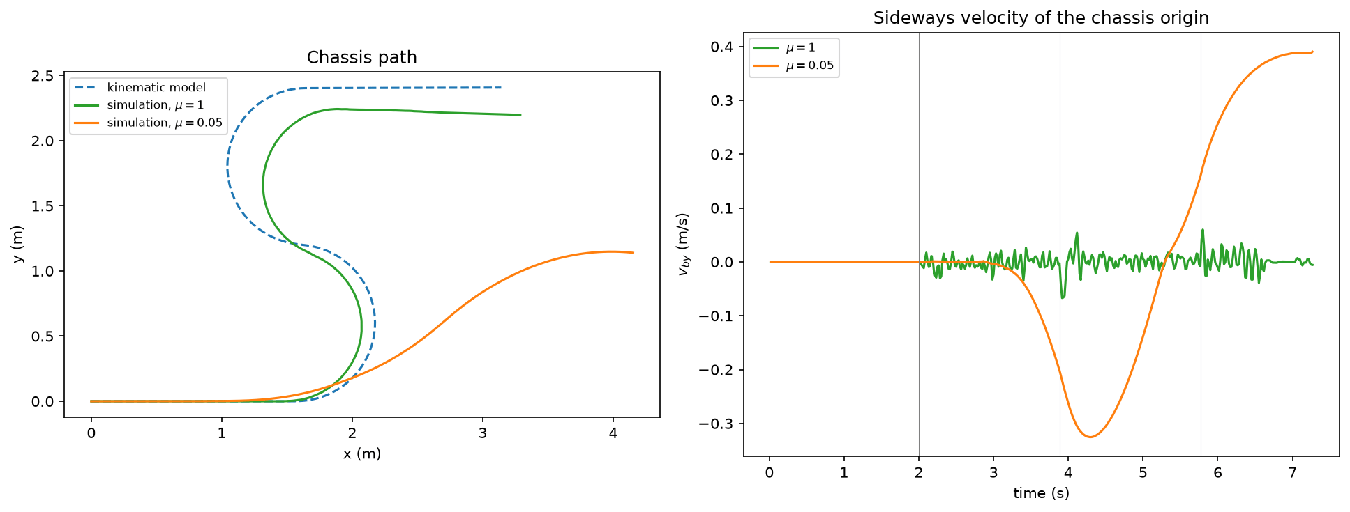

0.5\ \text{m/s}^2

DD_R, DD_D = 0.08, 0.18  # wheel radius r and half the distance between the wheels d


def build_diff_drive(mu):
    builder = newton.ModelBuilder()
    builder.default_joint_cfg.damping = 0.01
    # the chassis frame sits at the midpoint of the axle; the body extends backward to a ball caster
    chassis = builder.add_link(xform=wp.transform(p=wp.vec3(0.0, 0.0, DD_R), q=wp.quat_identity()), label="chassis")
    slick = newton.ModelBuilder.ShapeConfig(density=300.0, mu=1e-3, gap=0.01)
    builder.add_shape_box(chassis, xform=wp.transform(p=wp.vec3(-0.06, 0.0, 0.0), q=wp.quat_identity()),
                          hx=0.20, hy=0.13, hz=0.04, cfg=slick)
    builder.add_shape_sphere(chassis, xform=wp.transform(p=wp.vec3(-0.20, 0.0, -(DD_R - 0.03)), q=wp.quat_identity()),
                             radius=0.03, cfg=slick)
    joints, drives = [builder.add_joint_free(chassis)], []
    tire = newton.ModelBuilder.ShapeConfig(density=500.0, mu=mu, gap=0.01)
    axle_to_y = wp.quat_from_axis_angle(wp.vec3(1.0, 0.0, 0.0), -0.5 * wp.pi)
    for name, y in (("left", DD_D), ("right", -DD_D)):
        wheel = builder.add_link(label=name)
        builder.add_shape_cylinder(wheel, xform=wp.transform(q=axle_to_y), radius=DD_R, half_height=0.02, cfg=tire)
        drive = builder.add_joint_revolute(
            parent=chassis, child=wheel, parent_xform=wp.transform(p=wp.vec3(0.0, y, 0.0), q=wp.quat_identity()),
            child_xform=wp.transform(), axis=newton.Axis.Y, target_kd=40.0, damping=0.05, armature=0.02,
            effort_limit=80.0, actuator_mode=newton.JointTargetMode.VELOCITY, label=f"{name}_drive",
        )
        drives.append(drive)
        joints.append(drive)
    builder.add_articulation(joints)
    builder.add_ground_plane(cfg=newton.ModelBuilder.ShapeConfig(mu=mu, gap=0.01))
    return builder.finalize(), chassis, drives


def diff_drive_speeds(omega, v):
    return np.array([(v - DD_D * omega) / DD_R, (v + DD_D * omega) / DD_R])  # (u_L, u_R)


TURN_R, TURN_T = 0.6, np.pi * 0.6 / 1.0  # radius of each turn, and the time a half circle takes at 1 m/s
S_TIMES = (2.0, 2.0 + TURN_T, 2.0 + 2 * TURN_T)  # left turn starts, right turn starts, straight again


def s_curve(t):
    # (omega, v): straight, a half circle to the left, a half circle to the right, straight
    v = min(t / 1.0, 1.0)
    ease = lambda s: np.clip(s / 0.15, 0.0, 1.0)  # enter each turn over 0.15 s
    if S_TIMES[0] <= t < S_TIMES[1]:
        return v / TURN_R * ease(t - S_TIMES[0]), v
    if S_TIMES[1] <= t < S_TIMES[2]:
        return -v / TURN_R * ease(t - S_TIMES[1]), v
    return 0.0, v


T_S = S_TIMES[2] + 1.5
DT = 1.0 / 60
t_grid = np.arange(1, int(T_S * 60) + 1) * DT
model_path = integrate_twists([0.0, 0.0, 0.0], [(w, v, 0.0) for w, v in map(s_curve, t_grid)], DT)

t_dd, pose_grip, _ = simulate(*build_diff_drive(mu=1.0), lambda t: diff_drive_speeds(*s_curve(t)), duration=T_S)

def ice_frame(t, pose, angles):
    v_by = measured_body_twist(t[-3:], pose[-3:])[-1, 2] if len(t) > 2 else 0.0
    rr.log("plots/v_by", rr.Scalars(v_by))
    rr.log("paths/model", rr.LineStrips3D([path_strip(model_path)], colors=[[70, 130, 255]], radii=0.008), static=True)
    rr.log("paths/grip", rr.LineStrips3D([path_strip(pose_grip)], colors=[[60, 200, 90]], radii=0.008), static=True)
    rr.log("paths/ice", rr.LineStrips3D([path_strip(pose, z=0.02)], colors=[[255, 170, 0]], radii=0.01))


_, pose_ice, _ = simulate(*build_diff_drive(mu=0.05), lambda t: diff_drive_speeds(*s_curve(t)), duration=T_S,
                          recording=RECORDINGS / "diff-drive-0.41.rrd", on_frame=ice_frame, blueprint=layout("v_by"))

vby_grip = measured_body_twist(t_dd, pose_grip)[:, 2]
vby_ice = measured_body_twist(t_dd, pose_ice)[:, 2]
for name, pose, vby in (("mu = 1   ", pose_grip, vby_grip), ("mu = 0.05", pose_ice, vby_ice)):
    gap = np.hypot(pose[-1, 1] - model_path[-1, 1], pose[-1, 2] - model_path[-1, 2])
    print(f"{name}: max |v_by| = {np.abs(vby).max():.3f} m/s, final distance from the model's path = {gap:.2f} m")

mu = 1   : max |v_by| = 0.067 m/s, final distance from the model's path = 0.26 m
mu = 0.05: max |v_by| = 0.390 m/s, final distance from the model's path = 1.62 m

On the grippy floor,

v_{by}

stays near zero through both turns. Friction enforces the no-slip constraint assumed by the model, and the simulated path has the same shape as the model path. The turns are slightly tighter than the model’s because the effective wheel radius and track width differ a little from their nominal values. The odometry section measures these differences. On ice, friction cannot supply the sideways force needed for the turns. The chassis skids outward,

v_{by}

grows, and the robot ends up far from the predicted position. The no-slip assumption no longer holds.

The differential-drive robot on ice. The blue line is the kinematic model’s path and the green line the path on a grippy floor; the orange line traces the robot as it skids. The right-hand panel shows $v_{by}$ .

Odometry

Odometry estimates the chassis configuration by integrating wheel motion. Every wheeled robot can measure this motion with encoders. Between two readings, let

\Delta\varphi_L

and

\Delta\varphi_R

be the changes in the wheel angles. If the wheels turn at constant speed over the interval, the chassis moves at a constant body twist

\mathcal{V}_b = F \begin{bmatrix} \Delta\varphi_L \\ \Delta\varphi_R \end{bmatrix}, \qquad F = r \begin{bmatrix} -1/(2d) & 1/(2d) \\ 1/2 & 1/2 \\ 0 & 0 \end{bmatrix},

per unit time. The matrix exponential gives the exact displacement in

\{b\}

from integrating a constant twist for one unit of time. Rotate this displacement by the current heading, then add it to the current estimate to get the next estimate. The displace function above performs this calculation. The odometry estimate below uses the same function. Odometry errors accumulate because each step adds a new error to the previous ones. Some errors are systematic. Examples include a wheel radius or track width that differs from its nominal value. Calibration can remove these errors. Other errors, such as slip, are invisible to the encoders. The experiment below begins by calibrating the effective wheel radius from a straight run. It then calibrates the effective half track

d

from a steady circle. Both runs use the speed of the test drive. A wheel pressed into the floor rolls on a slightly smaller radius than its nominal one. It also touches the floor across the width of its tread. As a result, neither value matches the drawing. The robot then drives a long, winding path. The experiment compares the true path with three odometry estimates: nominal parameters on a grippy floor, calibrated parameters on the same floor, and calibrated parameters on ice. For each odometry update, you apply the discrete integration

\mathcal{X}_k = \mathcal{X}_{k-1} \oplus \tau_k

on SE(2), as described in calculus on Lie groups.

def odometry(q0, wheel_angles, r, d):
    F = r * np.array([[-1 / (2 * d), 1 / (2 * d)], [0.5, 0.5], [0.0, 0.0]])
    path = [np.asarray(q0, float)]
    for delta in np.diff(wheel_angles, axis=0):
        path.append(displace(path[-1], F @ delta, 1.0))
    return np.array(path)


# calibration runs at the speed of the test drive: straight ahead, then a steady circle
_, pose_s, ang_s = simulate(*build_diff_drive(mu=1.0), lambda t: diff_drive_speeds(0.0, 0.6 * min(t, 1.0)), duration=6.0)
k = len(pose_s) // 3  # skip the start, where the robot is still speeding up
r_eff = np.hypot(pose_s[-1, 1] - pose_s[k, 1], pose_s[-1, 2] - pose_s[k, 2]) / np.mean(ang_s[-1] - ang_s[k])
_, pose_c, ang_c = simulate(*build_diff_drive(mu=1.0), lambda t: diff_drive_speeds(0.6 * min(t, 1.0), 0.6 * min(t, 1.0)),
                            duration=8.0)
k = len(pose_c) // 4
turned = np.unwrap(pose_c[:, 0])[-1] - np.unwrap(pose_c[:, 0])[k]
d_eff = r_eff * ((ang_c[-1, 1] - ang_c[k, 1]) - (ang_c[-1, 0] - ang_c[k, 0])) / (2 * turned)
print(f"nominal    r = {DD_R:.4f} m, d = {DD_D:.4f} m")
print(f"calibrated r = {r_eff:.4f} m, d = {d_eff:.4f} m")


def winding(t):
    v = 0.6 * min(t / 1.0, 1.0)
    return 0.9 * np.sin(2 * np.pi * t / 12.0), v

nominal    r = 0.0800 m, d = 0.1800 m
calibrated r = 0.0766 m, d = 0.1849 m

def odometry_frame(t, pose, angles):
    # the calibrated estimate, advanced by the latest wheel-angle increment
    F = r_eff * np.array([[-1 / (2 * d_eff), 1 / (2 * d_eff)], [0.5, 0.5], [0.0, 0.0]])
    estimate = pose[0] if len(t) == 1 else displace(live[-1], F @ (angles[-1] - angles[-2]), 1.0)
    live.append(estimate)
    rr.log("paths/true", rr.LineStrips3D([path_strip(pose, z=0.02)], colors=[[255, 170, 0]], radii=0.01))
    rr.log("paths/odometry", rr.LineStrips3D([path_strip(np.array(live))], colors=[[70, 130, 255]], radii=0.008))
    rr.log("plots/position_error", rr.Scalars(float(np.hypot(*(estimate[1:] - pose[-1, 1:])))))


T_ODO = 36.0
live = []
t_o, pose_true, ang_true = simulate(*build_diff_drive(mu=1.0), lambda t: diff_drive_speeds(*winding(t)), duration=T_ODO,
                                    recording=RECORDINGS / "odometry-0.41.rrd", on_frame=odometry_frame,
                                    blueprint=layout("position_error"))

_, pose_ice_o, ang_ice_o = simulate(*build_diff_drive(mu=0.05), lambda t: diff_drive_speeds(*winding(t)), duration=T_ODO)

estimates = {
    "nominal r and d, grippy floor": (pose_true, odometry(pose_true[0], ang_true, DD_R, DD_D)),
    "calibrated r and d, grippy floor": (pose_true, odometry(pose_true[0], ang_true, r_eff, d_eff)),
    "calibrated r and d, ice": (pose_ice_o, odometry(pose_ice_o[0], ang_ice_o, r_eff, d_eff)),
}
errors = {k: np.hypot(est[:, 1] - true[:, 1], est[:, 2] - true[:, 2]) for k, (true, est) in estimates.items()}
for k, e in errors.items():
    print(f"{k:34s} error after {T_ODO:.0f} s: {e[-1]:.3f} m")

nominal r and d, grippy floor      error after 36 s: 2.016 m
calibrated r and d, grippy floor   error after 36 s: 1.051 m
calibrated r and d, ice            error after 36 s: 4.156 m

With nominal parameters, the error grows steadily. Each wheel revolution is converted to distance with a slightly incorrect radius. Each turn is converted to heading with a slightly incorrect track width. Calibration reduces this systematic error substantially, but some error remains. A single pair of values for

r

and

d

cannot match every part of a winding drive. On ice, the calibrated estimate fails again. The wheels turn, but the chassis does not move as their motion indicates. No choice of

r

and

d

can account for this slip. Robots therefore combine odometry, which is accurate over short times, with sensors whose errors do not accumulate. These may include range sensors, cameras or GPS. An estimator such as a Kalman filter combines the measurements. The state estimation and mapping chapter develops these methods.

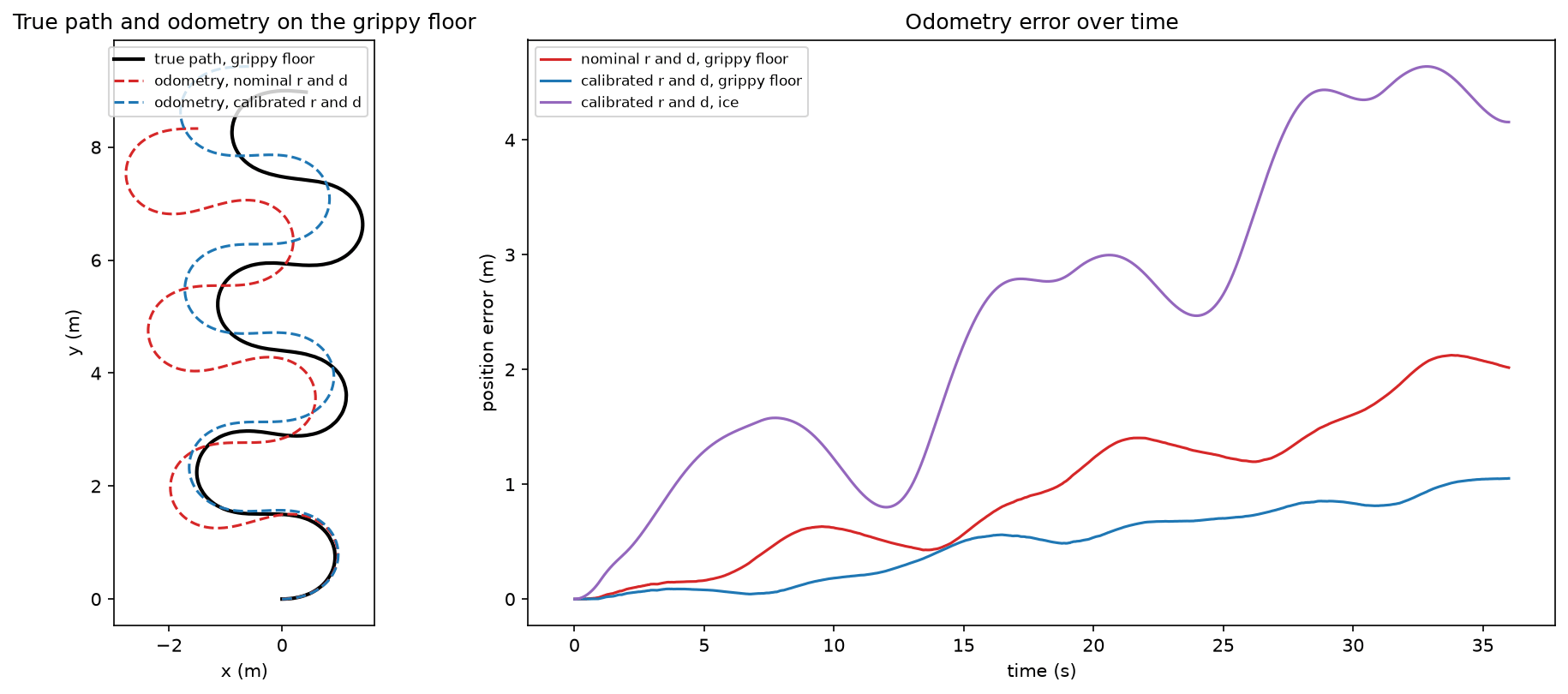
The winding drive on the grippy floor. The orange line is the true path and the blue line the calibrated odometry estimate; the right-hand panel shows their distance over time.

Further topics

Chapter 13 of Lynch and Park also covers the controllability of nonholonomic robots, including why a car can parallel park even though it cannot move sideways. It discusses motion planning under nonholonomic constraints, including shortest paths for a car with a minimum turning radius. It also treats feedback control for tracking a reference trajectory and mobile manipulation, where an arm is mounted on a wheeled base. The planning lectures in this course cover path planning for mobile robots.

References

Kevin M. Lynch, F. (2017). Modern Robotics.
(n.d.). Data Curation for Machine Learning.

Found an error on this page? Report an issue.

Robotics Systems

Motion Algebras

Kinematics

Dynamics

Systems Integration

Nonholonomic Wheeled Robots

Simulating the robot

Nonholonomic robots

Wheel speeds of a differential drive

Odometry

Further topics

References

​Simulating the robot

​Nonholonomic robots

​Wheel speeds of a differential drive

​Odometry

​Further topics

​References

Simulating the robot

Nonholonomic robots

Wheel speeds of a differential drive

Odometry

Further topics

References