

 The previous section
built the AR4 analytically from its Denavit-Hartenberg table. This lab takes the same arm from
the other end: its URDF, the as-built description that drives the live Gazebo simulation of
the AR4 physical-AI project. You read the
kinematic chain straight out of the file, compute forward kinematics from it, reconcile the
result against the DH model, map the reachable workspace, and solve position inverse kinematics.
The same forward-kinematics code was used on the project to diagnose why a vision-language-action
policy’s grasps were missing: forward-mapping what the policy commanded into Cartesian space and
asking where the hand actually went.
The previous section
built the AR4 analytically from its Denavit-Hartenberg table. This lab takes the same arm from
the other end: its URDF, the as-built description that drives the live Gazebo simulation of
the AR4 physical-AI project. You read the
kinematic chain straight out of the file, compute forward kinematics from it, reconcile the
result against the DH model, map the reachable workspace, and solve position inverse kinematics.
The same forward-kinematics code was used on the project to diagnose why a vision-language-action
policy’s grasps were missing: forward-mapping what the policy commanded into Cartesian space and
asking where the hand actually went.
fixed attachments (covers, motors, the wrist camera). A URDF is a tree; the chain
from the base to any link is recovered by walking child→parent:
Forward kinematics
Each URDF joint contributes two transforms: a fixed origin (translation , then a roll-pitch-yaw rotation) and, for actuated joints, a motion about/along its axis by the joint variable : with given by the axis-angle (Rodrigues) formula. FK is the ordered product along the chain: .
Frame caveat from practice. These coordinates are in the robot’s base_link frame. In
the project’s Gazebo world the base is yawed 90°, so ,
: forgetting this cost us an afternoon when comparing FK output
against ground-truth object poses.
Reconciling the URDF with the DH model
The two descriptions are of one physical arm, so the parts that encode geometry must agree, and the parts that encode a coordinate convention are free to differ. Separating the two is the practical skill. Converting the URDF’s metres to millimetres and reading the link lengths off the joint origins lines them up against the DH table: the upper arm and the tool offset match exactly, the shoulder offset to a twentieth of a millimetre. One number does not: the forearm reads 222.63 mm in the DH table and 222.94 mm in the URDF, a genuine 0.31 mm gap between the nominal calibration and the CAD-derived model that no change of frame removes. The tool positions at the zero pose, by contrast, differ completely, because the two models define the zero configuration through different conventions (the URDF through each joint-origin roll-pitch-yaw, the DH table through its angle-offset column). Making the positions coincide takes an explicit base transform and a per-joint sign and offset map, which is bookkeeping, not physics.The reachable workspace
Sampling joint vectors uniformly inside the URDF limits and plotting the grasp center for each gives an honest picture of where the hand can actually go. The red marker is the home pose.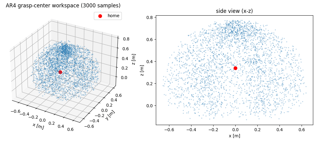
Inverse kinematics: position by damped least squares
Position inverse kinematics asks: find such that , where is the forward kinematics above. Linearize with the Jacobian (estimated here by finite differences) and iterate the damped least-squares update, which stays well behaved near singularities where the plain pseudo-inverse blows up: This solves for position only. The previous section solved the full six-dimensional pose, position and orientation together, by stacking an orientation error under the position error and growing to .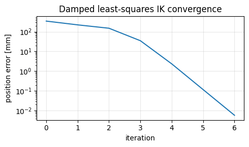
Found an error on this page? Report an issue.