Rotation representations

This section draws from section 3.2, Rotations and Angular Velocities, of Kevin Lynch and Frank Park, Modern Robotics: Mechanics, Planning, and Control (Kevin M. Lynch, 2017). You can download the chapter as a PDF. A rigid body in space has six degrees of freedom: three for position and three for orientation. A body in the plane has three: two for position and one for orientation. This section describes orientation and its change over time. It begins with the general case in three dimensions. Each part then treats the plane as a special case in a paragraph marked In the plane. These paragraphs also provide background for wheeled robots.

​

Vectors and reference frames

A free vector $\mathbf{v} \in \mathbb{R}^n$ is a geometric quantity with magnitude and direction. It does not depend on a coordinate system. It acquires numerical values when you express it in a coordinate frame. For example, a velocity vector may be $\mathbf{v} = [3, 1, 0]^T$ in frame $\{a\}$ and have different coordinates in frame $\{b\}$. You can also represent points as vectors. Their coordinates are measured from the origin of a reference frame, as shown below. A point and a free vector behave differently when the frame changes. The coordinates of a point depend on the frame’s origin. A free vector is unaffected by translation and only rotates. Homogeneous coordinates show this distinction by appending a 1 to a point and a 0 to a free vector.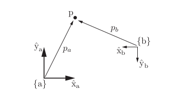 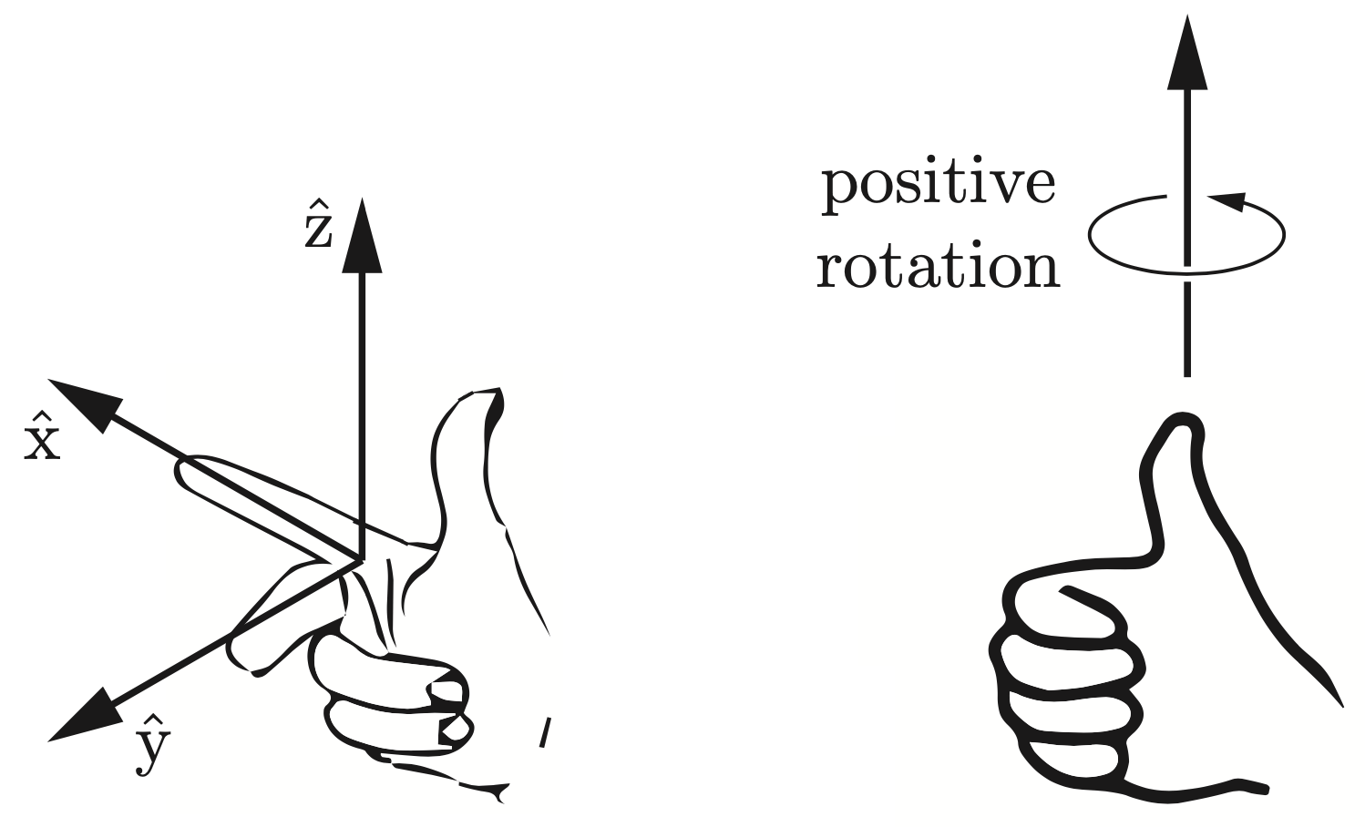All frames here are right handed and inertial, meaning that they do not accelerate or rotate. A frame fixed to the ground turns with the Earth, but this effect is small enough to ignore for robots. Rigid-body dynamics explains what changes in an accelerating frame. The unit axes of every frame follow the right-hand rule and satisfy $\hat x \times \hat y = \hat z$. Point your right thumb along an axis. The curled fingers give the direction of positive rotation about that axis. We define one fixed frame, the space frame $\{s\}$. It is also called the world frame. We also define a body frame $\{b\}$ associated with the body. At each instant, this frame coincides with the frame attached to the body. Lynch and Park use only inertial frames. Their body frame $\{b\}$ does not move with the body. At a given instant, it is the stationary frame aligned with the frame attached to the body.

• The body can accelerate, and its attached frame moves with it.
• Velocities are always measured relative to inertial space.

• Each instant uses a new stationary body frame. This frame is aligned with the body at that instant.

Every frame used by Lynch and Park is therefore inertial, so their derivations contain no fictitious forces.

​

Rotation matrices

The rotation matrices form the special orthogonal group $SO(3)$. The product of two rotation matrices is another rotation matrix, $R_1 R_2 \in SO(3)$. Every rotation matrix has an inverse, $R^{-1} = R^\top$. Rotations preserve lengths, $\|Rv\| = \|v\|$.

​

In the plane

Begin in the plane, where a frame has two axes. In the figure below, the body frame $\{b\}$ has its origin at $\mathbf{p}$ and is rotated by an angle $\theta$ relative to the space frame 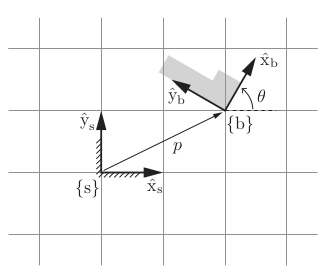$\{s\}$. Write each body axis in space-frame coordinates: $$\hat{x}_b = \cos\theta\, \hat{x}_s + \sin\theta\, \hat{y}_s, \qquad \hat{y}_b = -\sin\theta\, \hat{x}_s + \cos\theta\, \hat{y}_s .$$ Place these vectors side by side as columns. The result is a rotation matrix: $$R(\theta) = \begin{bmatrix} \hat{x}_b & \hat{y}_b \end{bmatrix} = \begin{bmatrix} \cos\theta & -\sin\theta \\ \sin\theta & \cos\theta \end{bmatrix} \in SO(2) .$$ The columns are perpendicular unit vectors. Their four entries obey three constraints: two unit-length conditions and one orthogonality condition. One free number remains, the angle $\theta$. SO(2) as a manifold studies this group in detail.

​

In space

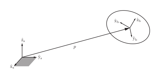
A frame in space has three axes, but the construction is unchanged. Let $\mathbf{p}$ denote the vector from the fixed-frame origin to the body-frame origin. In fixed-frame coordinates, $$\mathbf{p} = p_1 \, \hat{\mathbf{x}}_s + p_2 \, \hat{\mathbf{y}}_s + p_3 \, \hat{\mathbf{z}}_s . \tag{3.12}$$ You can also express the axes of the body frame in the fixed frame: $$\begin{aligned} \hat{\mathbf{x}}_b &= r_{11} \hat{\mathbf{x}}_s + r_{21} \hat{\mathbf{y}}_s + r_{31} \hat{\mathbf{z}}_s \\ \hat{\mathbf{y}}_b &= r_{12} \hat{\mathbf{x}}_s + r_{22} \hat{\mathbf{y}}_s + r_{32} \hat{\mathbf{z}}_s \\ \hat{\mathbf{z}}_b &= r_{13} \hat{\mathbf{x}}_s + r_{23} \hat{\mathbf{y}}_s + r_{33} \hat{\mathbf{z}}_s \end{aligned}$$ Place these three vectors side by side as columns. The result is a $3 \times 3$ rotation matrix: $$\mathbf{p} = \begin{bmatrix} p_1 \\ p_2 \\ p_3 \end{bmatrix}, \qquad R = \begin{bmatrix} r_{11} & r_{12} & r_{13} \\ r_{21} & r_{22} & r_{23} \\ r_{31} & r_{32} & r_{33} \end{bmatrix} = \begin{bmatrix} \hat{\mathbf{x}}_b & \hat{\mathbf{y}}_b & \hat{\mathbf{z}}_b \end{bmatrix} .$$ The pair $(R, \mathbf{p})$ contains 12 parameters and fully describes the body’s position and orientation relative to the fixed frame. A rotation matrix has three uses (Lynch and Park section 3.2.1, book pages 66 to 69):

• It represents an orientation. Its columns give the directions of the body axes.
• It changes coordinates. A vector $v_b$ written in the body frame has coordinates $v_s = R\,v_b$ in the world frame. For example, a robot that drives forward along its heading moves in the world direction given by the first column of $R$.
• It rotates vectors and frames. The vector $R\,v$ is $v$ rotated by the orientation described by $R$.

A general matrix is not a rotation matrix. Its columns must be perpendicular unit vectors. These requirements give six equations for the nine entries and can be written as $R^\top R = I$ (Lynch and Park eq. 3.19). A right-handed frame also requires $\det R = 1$ (eq. 3.21). A matrix with $\det R = -1$ describes a reflection. The six constraints leave three free numbers, matching the three degrees of freedom of an orientation in space. The planar $R(\theta)$ is a rotation about $\hat z$ with the third row and column removed.

​

Angular velocity

Suppose a frame with unit axes $\{\hat{x}, \hat{y}, \hat{z}\}$ is attached to a rotating body. Consider the time derivatives of these axes. The length of $\hat{x}$ is fixed, so only its direction can change. The same is true of $\hat{y}$ and $\hat{z}$. Between times $t$ and $t + \Delta t$, the orientation changes by a rotation through an angle $\Delta \theta$ about a unit axis $\hat{\omega}$ through the origin. The axis $\hat{\omega}$ is independent of coordinates and has not yet been expressed in a reference frame. As $\Delta t$ approaches zero, the ratio $\Delta \theta / \Delta t$ approaches the rotation rate $\dot{\theta}$. The vector $\hat{\omega}$ becomes the instantaneous axis of rotation. Together they define the angular velocity $$\omega = \hat{\omega} \, \dot{\theta} .$$ Each unit axis moves with velocity $\omega \times \hat{x}$, which is perpendicular to both $\omega$ and $\hat{x}$. This animation follows Figure 3.10 of Lynch and Park. During $\Delta t$, the frame turns by $\Delta\theta$ about $\hat{\omega}$. In the limit, $\omega = \hat{\omega}\dot\theta$, and the tip of $\hat{x}$ has velocity $\omega \times \hat{x}$. The final view places the axis along the plane normal $\hat{z}$ to show the planar case. Angular velocity provides a familiar example of a quantity in a Lie algebra. A point on a rotating body has velocity $v = \omega \times r$. The cross product with $\omega$ is a linear map, so you can write it as $v = [\omega]\,r$. For a vector $\mathbf{x} \in \mathbb{R}^3$, $$[\mathbf{x}] = \begin{bmatrix} 0 & -x_3 & x_2 \\ x_3 & 0 & -x_1 \\ -x_2 & x_1 & 0 \end{bmatrix} , \qquad [\mathbf{x}] = -[\mathbf{x}]^T .$$ The set of all $3 \times 3$ real skew-symmetric matrices is $\mathfrak{so}(3)$. The matrix $[\omega]$ is the hat of $\omega$ and belongs to this Lie algebra. Let $R(t)$ describe the orientation of the body frame relative to the fixed frame at time $t$. Its columns $\mathbf{r}_1(t)$, $\mathbf{r}_2(t)$ and $\mathbf{r}_3(t)$ give $\hat{x}$, $\hat{y}$ and $\hat{z}$ in fixed-frame coordinates. Let $\omega_s$ be the angular velocity expressed in the fixed frame. Each column then moves according to $$\dot{\mathbf{r}}_i = \omega_s \times \mathbf{r}_i , \qquad i = 1, 2, 3 ,$$ so $\dot R = [\omega_s] R$. Page 79 of Lynch and Park solves this equation for the angular velocity. In fixed-frame and body-frame coordinates, $$[\omega_s] = \dot{R} R^{-1} , \qquad [\omega_b] = R^{-1} \dot{R} ,$$ with $R^{-1} = R^\top$. The second form is the $\mathcal{X}^{-1}\dot{\mathcal{X}}$ of Lie I. The fixed-frame angular velocity $\omega_s$ is independent of the chosen body frame. Similarly, the body-frame angular velocity $\omega_b$ is independent of the chosen fixed frame. Both $R$ and $\dot{R}$ depend on $\{s\}$ and $\{b\}$. Their products remove one of these dependencies. The product $\dot{R} R^{-1}$ is independent of $\{b\}$, while $R^{-1} \dot{R}$ is independent of $\{s\}$. In the plane. Every rotation is about the axis perpendicular to the plane, so angular velocity is the scalar $\omega = \dot\theta$. Differentiating $R(\theta)$ gives $\dot R = [\omega] R$, where $$[\omega] = \begin{bmatrix} 0 & -\omega \\ \omega & 0 \end{bmatrix} \in \mathfrak{so}(2)$$ is the skew-symmetric matrix that appears as the tangent at the identity in SO(2) as a manifold. Because planar rotations commute, $\omega_s = \omega_b = \dot\theta$.

​

Exponential coordinates

You can also write a rotation as an exponential. Suppose a body rotates with constant unit angular velocity $\hat\omega$ for a time $\theta$. Its orientation obeys $\dot R = [\hat\omega] R$. This linear differential equation has the solution $R(\theta) = e^{[\hat\omega]\theta} R(0)$. The matrix exponentials used by Lynch and Park, $e^{[\hat\omega]\theta}$ for rotations and $e^{[\mathcal{S}]\theta}$ for rigid motions, are instances of the Lie exponential from Lie I. The product of exponentials formula for robot arms is named for its product of Lie-group exponentials. A rotation by an angle $\theta$ about a unit axis $\hat\omega$ is described by the three numbers $\hat\omega\theta \in \mathbb{R}^3$, called its exponential coordinates. Let $[\hat\omega]$ be the skew-symmetric matrix of $\hat\omega$ from angular velocity. Rodrigues’ formula computes the rotation matrix. This formula is the exponential map Exp of SO(3): $$R = e^{[\hat\omega]\theta} = I + \sin\theta\, [\hat\omega] + (1 - \cos\theta)[\hat\omega]^2 .$$ The logarithm of a rotation inverts the matrix exponential for rotation angles $0 \le \theta < \pi$. Rotations by $\theta$ and $\theta + 2\pi$ produce the same matrix, so a single inverse cannot cover every angle. A rotation by exactly $\pi$ requires separate treatment. The axes $\hat{\omega}$ and $-\hat{\omega}$ produce the same rotation, so the logarithm has two solutions and needs a sign convention. For $\theta = 0$ the logarithm is the zero matrix. If $0 < \theta < \pi$, then $$[\hat\omega] = \frac{1}{2 \sin \theta}(R - R^T) .$$ SO(3) is a curved three-dimensional space. Its exponential map wraps a flat coordinate space onto it. You cannot draw a curved three-dimensional space, but the unit sphere $S^2$ shows the same structure in one lower dimension. At a point $p$, the tangent plane $T_pS^2$ touches the sphere and contains every possible velocity of a curve through $p$. The exponential map carries a tangent vector $\omega$ onto the sphere. It follows the great circle in the vector’s direction for an arc length $\|\omega\|$: $$\exp_p(\omega) = \cos(\|\omega\|)\, p + \sin(\|\omega\|)\, \frac{\omega}{\|\omega\|}$$ Straight lines in the tangent plane become curved arcs on the sphere. Near $p$, the plane approximates the sphere well. SO(3) has the same local structure. Its tangent space is $\mathbb{R}^3$, and the exponential map turns a vector $\hat{\omega}\theta$ into a rotation matrix. The sphere provides a visible model of SO(3). The gold plane is the tangent plane $T_pS^2$ at $p$, and the white arrow is a tangent vector $\omega$. The red arc is $\exp_p(\omega)$, the great-circle path that starts at $p$, follows the direction of $\omega$, and has the same length. The fan shows this mapping in twelve directions. The final orbit compares the flat plane with arcs that follow the sphere’s curvature. In the plane. Rotations in SO(2) commute, which makes the planar case simpler. A rotation by $\alpha$ followed by one through $\beta$ gives the same result in reverse order. The angles simply add. Spatial rotations do not commute, as the following example shows. First rotate a frame by $90^\circ$ about the fixed $x$ axis, then rotate it by $90^\circ$ about the fixed $y$ axis: $$R_y R_x = \begin{bmatrix} 0 & 0 & 1 \\ 0 & 1 & 0 \\ -1 & 0 & 0 \end{bmatrix} \begin{bmatrix} 1 & 0 & 0 \\ 0 & 0 & -1 \\ 0 & 1 & 0 \end{bmatrix} = \begin{bmatrix} 0 & 1 & 0 \\ 0 & 0 & -1 \\ -1 & 0 & 0 \end{bmatrix} .$$ Reverse the order: $$R_x R_y = \begin{bmatrix} 0 & 0 & 1 \\ 1 & 0 & 0 \\ 0 & 1 & 0 \end{bmatrix} .$$ The results differ. In the first case, the frame’s $x$ axis points along $-z$. In the second, it points along $+y$. You therefore cannot add 3-D rotation coordinates directly. The adjoint and Lie bracket from calculus on Lie groups account for the order of the rotations. In the plane, every rotation is about $\hat z$, so the axis is fixed and the exponential coordinates reduce to the angle $\theta$. With $[\hat z]$ restricted to the plane, Rodrigues’ formula becomes $e^{\theta G} = I\cos\theta + G\sin\theta = R(\theta)$, where $G$ is the quarter-turn matrix of Lie I.

​

Other representations

Robotics uses several representations of orientation: rotation matrices, axis-angle coordinates, exponential coordinates, Euler angles, and quaternions. The choice depends on the application, the vendor and the software tools. Aeronautics and self-driving cars may use different conventions because of the robots involved or the history of each field. The discussion of Euler angles and quaternions below draws from Introduction to Autonomous Robots.

​

Euler angles

Three values suffice to describe orientation. Orthogonality and unit vector length impose six constraints on the nine entries of a rotation matrix. You can therefore represent an orientation by rotations through specified angles about the $x$, $y$, and $z$ axes of the reference coordinate system. This representation is called X-Y-Z fixed-angle notation. Its rotation matrix is $^s_BR_{XYZ}(\gamma,\beta,\alpha)=\begin{bmatrix}\cos\alpha & -\sin\alpha & 0\\ \sin\alpha & \cos\alpha & 0\\0 & 0 & 1\end{bmatrix}\begin{bmatrix}\cos\beta& 0 & \sin\beta\\0 & 1 & 0\\-\sin\beta & 0 & \cos\beta\end{bmatrix}\begin{bmatrix}1 & 0 & 0 \\ 0 & \cos\gamma & -\sin\gamma\\0 & \sin\gamma & \cos\gamma\end{bmatrix}$ X-Y-Z fixed angles express a coordinate frame using rotations relative to the original frame $\{A\}$. You can describe the same sequence by starting with a frame $\{B\}$ that coincides with $\{A\}$. Rotate it about the Z-axis by $\alpha$, the Y-axis by $\beta$, and the X-axis by $\gamma$. This representation is called Z-Y-X Euler angles. The coordinate axes need not all differ. There are twelve valid rotation sequences: XYX, XZX, YXY, YZY, ZXZ, ZYZ, XYZ, XZY, YZX, YXZ, ZXY, and ZYX. Consecutive rotations about the same axis are excluded because they are equivalent to one rotation through the sum of the angles. Different applications use different conventions. Hardware and software manufacturers often choose conventions based on the fields for which their products were developed, such as aviation or geology. These representations become singular at certain angle values. At a singularity, a sequence can be equivalent to consecutive rotations about the same axis. For example, the XYZ rotation matrix is singular when the angle about the Y-axis is 90°. Other representations avoid these singularities over the full range of possible motions.

​

Quaternions

Quaternions represent a rotation with four numbers. They can be composed at low computational cost and normalized with little effort. They also avoid gimbal lock. Most robot software therefore uses them to represent orientation. Quaternions from complex numbers derives the representation from vector rotation through the double cover of SO(3). The Lie cheatsheet collects these representations and their velocity counterparts in tables.

​

References

• Kevin M. Lynch, F. (2017). Modern Robotics.

---