Exact Solution (not recommended)
Suppose we have two states: S={s1,s2}, and a deterministic policy π that always chooses action a. The dynamics are:- From s1, action leads to s2 with reward 2
- From s2, action leads to s1 with reward 0
- Reward vector:
Iterative Policy Evaluation
This method is based on the recognition that the Bellman operator is contractive. We can apply the Bellman expectation backup equations repeatedly in an iterative fashion and converge to the state-value function of the policy. We start at k=0 by initializing all state-value function (a vector) to v0(s)=0. In each iteration k we start with the state value function of the previous iteration vk(s) and apply the Bellman expectation backup as prescribed by the one step lookahead tree below that is decorated relative to what we have seen in the Bellman expectation backup with the iteration information. This is called the synchronous backup formulation as we are updating all the elements of the value function vector at the same time.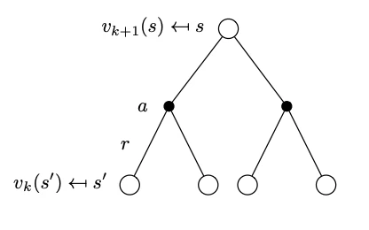
A simple scalar contraction that illustrates the idea behind iterative policy evaluation is:xk+1=c+γxkwhere:This will converge to x=1−0.92=20.
- c is a constant (analogous to reward),
- γ∈[0,1) is the contraction factor (analogous to the discount factor in MDPs).
# Scalar contraction example
c = 2
gamma = 0.9
x = 0

print("Scalar contraction iterations:\n")
for i in range(10):
    x = c + gamma * x
    print(f"Iteration {i+1}: x = {x}")
Policy Evaluation - Minigrid Examples
The following examples are based on the minigrid - empty environment.import numpy as np
import gymnasium as gym
from minigrid.wrappers import FullyObsWrapper
from copy import deepcopy
from collections import deque
import hashlib
import json
def build_minigrid_model(env):
"""
Enumerate all reachable fully-observable states in MiniGrid,
then build P[s,a,s'] and R[s,a]
"""
# wrap to get full grid observation (no partial obs)
env = FullyObsWrapper(env)
# helper to hash an obs dictionary
def obs_key(o):
if isinstance(o, dict):
# For dictionary observations, extract the 'image' part which is the grid
if "image" in o:
return o["image"].tobytes()
else:
# If no 'image' key, convert dict to a stable string representation
return hashlib.md5(
json.dumps(str(o), sort_keys=True).encode()
).hexdigest()
else:
# For array observations (older versions)
return o.tobytes()
# BFS over states
state_dicts = [] # index -> env.__dict__ snapshot
obs_to_idx = {} # obs_key -> index
transitions = {} # (s,a) -> (s', r, done)
# init
obs, _ = env.reset(seed=0)
idx0 = 0
obs_to_idx[obs_key(obs)] = idx0
state_dicts.append(deepcopy(env.unwrapped.__dict__))
queue = deque([obs])
while queue:
obs = queue.popleft()
s = obs_to_idx[obs_key(obs)]
# restore that state
env.unwrapped.__dict__.update(deepcopy(state_dicts[s]))
for a in range(env.action_space.n):
obs2, r, terminated, truncated, _ = env.step(a)
done = terminated or truncated
key2 = obs_key(obs2)
if key2 not in obs_to_idx:
obs_to_idx[key2] = len(state_dicts)
state_dicts.append(deepcopy(env.unwrapped.__dict__))
queue.append(obs2)
s2 = obs_to_idx[key2]
transitions[(s, a)] = (s2, r, done)
# restore before next action
env.unwrapped.__dict__.update(deepcopy(state_dicts[s]))
nS = len(state_dicts)
nA = env.action_space.n
# build P and R arrays
P = np.zeros((nS, nA, nS), dtype=np.float32)
R = np.zeros((nS, nA), dtype=np.float32)
for (s, a), (s2, r, done) in transitions.items():
if done:
# absorbing: stay in s
P[s, a, s] = 1.0
else:
P[s, a, s2] = 1.0
R[s, a] = r
return P, R, state_dicts
Exact Solution (not recommended)
def solve_policy_linear_minigrid(env, gamma=0.9):
    """
    Under uniform random policy, solve (I - γ P^π) v = R^π exactly.
    """
    P, R, state_dicts = build_minigrid_model(env)
    nS, nA = R.shape

    # uniform random policy
    pi = np.ones((nS, nA)) / nA

    # build P^π and R^π
    P_pi = np.einsum(
        "sa,sab->sb", pi, P
    )  # shape (nS,nS) - fixed indices to avoid repeated output subscript
    R_pi = (pi * R).sum(axis=1)  # shape (nS,)

    # solve linear system
    A = np.eye(nS) - gamma * P_pi
    v = np.linalg.solve(A, R_pi)
    return v, state_dicts


if __name__ == "__main__":
    # 1. create the Minigrid env
    env = gym.make("MiniGrid-Empty-5x5-v0")

    # 2. solve for v under random policy
    v, states = solve_policy_linear_minigrid(
        env, gamma=0.99
    )  # Changed from 1.0 to 0.99

    # 3. print out values by (pos,dir)
    print("State-value function for each (x,y,dir):\n")
    for idx, sdict in enumerate(states):
        pos = sdict["agent_pos"]
        d = sdict["agent_dir"]
        print(f"  s={idx:2d}, pos={pos}, dir={d}:  V = {v[idx]:6.3f}")
State-value function for each (x,y,dir):

  s= 0, pos=(1, 1), dir=0:  V =  0.924
  s= 1, pos=(1, 1), dir=3:  V =  0.863
  s= 2, pos=(1, 1), dir=1:  V =  0.923
  s= 3, pos=(np.int64(2), np.int64(1)), dir=0:  V =  1.051
  s= 4, pos=(1, 1), dir=2:  V =  0.863
  s= 5, pos=(np.int64(1), np.int64(2)), dir=1:  V =  1.049
  s= 6, pos=(np.int64(2), np.int64(1)), dir=3:  V =  0.961
  s= 7, pos=(np.int64(2), np.int64(1)), dir=1:  V =  1.061
  s= 8, pos=(np.int64(3), np.int64(1)), dir=0:  V =  1.205
  s= 9, pos=(np.int64(1), np.int64(2)), dir=0:  V =  1.061
  s=10, pos=(np.int64(1), np.int64(2)), dir=2:  V =  0.960
  s=11, pos=(np.int64(1), np.int64(3)), dir=1:  V =  1.200
  s=12, pos=(np.int64(2), np.int64(1)), dir=2:  V =  0.940
  s=13, pos=(np.int64(2), np.int64(2)), dir=1:  V =  1.268
  s=14, pos=(np.int64(3), np.int64(1)), dir=3:  V =  1.122
  s=15, pos=(np.int64(3), np.int64(1)), dir=1:  V =  1.373
  s=16, pos=(np.int64(1), np.int64(2)), dir=3:  V =  0.939
  s=17, pos=(np.int64(2), np.int64(2)), dir=0:  V =  1.270
  s=18, pos=(np.int64(1), np.int64(3)), dir=0:  V =  1.367
  s=19, pos=(np.int64(1), np.int64(3)), dir=2:  V =  1.118
  s=20, pos=(np.int64(2), np.int64(2)), dir=2:  V =  1.077
  s=21, pos=(np.int64(2), np.int64(3)), dir=1:  V =  1.547
  s=22, pos=(np.int64(3), np.int64(1)), dir=2:  V =  1.118
  s=23, pos=(np.int64(3), np.int64(2)), dir=1:  V =  1.893
  s=24, pos=(np.int64(2), np.int64(2)), dir=3:  V =  1.077
  s=25, pos=(np.int64(3), np.int64(2)), dir=0:  V =  1.555
  s=26, pos=(np.int64(1), np.int64(3)), dir=3:  V =  1.115
  s=27, pos=(np.int64(2), np.int64(3)), dir=0:  V =  1.882
  s=28, pos=(np.int64(2), np.int64(3)), dir=2:  V =  1.322
  s=29, pos=(np.int64(3), np.int64(2)), dir=2:  V =  1.399
  s=30, pos=(np.int64(3), np.int64(3)), dir=1:  V =  1.088
  s=31, pos=(np.int64(3), np.int64(2)), dir=3:  V =  1.327
  s=32, pos=(np.int64(2), np.int64(3)), dir=3:  V =  1.394
  s=33, pos=(np.int64(3), np.int64(3)), dir=0:  V =  1.089
  s=34, pos=(np.int64(3), np.int64(3)), dir=2:  V =  1.165
  s=35, pos=(np.int64(3), np.int64(3)), dir=3:  V =  1.166
Iterative Method
import numpy as np
import gymnasium as gym
from minigrid.wrappers import FullyObsWrapper


def policy_eval_iterative(env, policy, discount_factor=0.99, epsilon=0.00001):
    """
    Evaluate a policy given an environment using iterative policy evaluation.

    Args:
        policy: [S, A] shaped matrix representing the policy.
        env: MiniGrid environment
        discount_factor: Gamma discount factor.
        epsilon: Threshold for convergence.

    Returns:
        Vector representing the value function.
    """
    # Build model to get state space size and transition probabilities
    P, R, state_dicts = build_minigrid_model(env)
    nS, nA = R.shape

    # Start with zeros for the value function
    V = np.zeros(nS)

    while True:
        delta = 0
        # For each state, perform a "full backup"
        for s in range(nS):
            v = 0
            # Look at the possible next actions
            for a, action_prob in enumerate(policy[s]):
                # For each action, look at the possible next states
                for s_next in range(nS):
                    # If transition is possible
                    if P[s, a, s_next] > 0:
                        # Calculate the expected value
                        v += (
                            action_prob
                            * P[s, a, s_next]
                            * (R[s, a] + discount_factor * V[s_next])
                        )
            # How much did the value change?
            delta = max(delta, np.abs(v - V[s]))
            V[s] = v
        # Stop evaluating once our value function change is below threshold
        if delta < epsilon:
            break

    return V


# Create the MiniGrid environment
env = gym.make("MiniGrid-Empty-5x5-v0")
env = FullyObsWrapper(env)

# Get model dimensions
P, R, state_dicts = build_minigrid_model(env)
nS, nA = R.shape

# Create a uniform random policy
random_policy = np.ones([nS, nA]) / nA

# Evaluate the policy
v = policy_eval_iterative(env, random_policy, discount_factor=0.99)

# Print results
print("State-value function using iterative policy evaluation:\n")
for idx, sdict in enumerate(state_dicts):
    pos = sdict["agent_pos"]
    d = sdict["agent_dir"]
    print(f"  s={idx:2d}, pos={pos}, dir={d}:  V = {v[idx]:6.3f}")
State-value function using iterative policy evaluation:

  s= 0, pos=(1, 1), dir=0:  V =  0.923
  s= 1, pos=(1, 1), dir=3:  V =  0.862
  s= 2, pos=(1, 1), dir=1:  V =  0.923
  s= 3, pos=(np.int64(2), np.int64(1)), dir=0:  V =  1.050
  s= 4, pos=(1, 1), dir=2:  V =  0.862
  s= 5, pos=(np.int64(1), np.int64(2)), dir=1:  V =  1.048
  s= 6, pos=(np.int64(2), np.int64(1)), dir=3:  V =  0.961
  s= 7, pos=(np.int64(2), np.int64(1)), dir=1:  V =  1.060
  s= 8, pos=(np.int64(3), np.int64(1)), dir=0:  V =  1.204
  s= 9, pos=(np.int64(1), np.int64(2)), dir=0:  V =  1.060
  s=10, pos=(np.int64(1), np.int64(2)), dir=2:  V =  0.959
  s=11, pos=(np.int64(1), np.int64(3)), dir=1:  V =  1.199
  s=12, pos=(np.int64(2), np.int64(1)), dir=2:  V =  0.939
  s=13, pos=(np.int64(2), np.int64(2)), dir=1:  V =  1.267
  s=14, pos=(np.int64(3), np.int64(1)), dir=3:  V =  1.121
  s=15, pos=(np.int64(3), np.int64(1)), dir=1:  V =  1.372
  s=16, pos=(np.int64(1), np.int64(2)), dir=3:  V =  0.938
  s=17, pos=(np.int64(2), np.int64(2)), dir=0:  V =  1.269
  s=18, pos=(np.int64(1), np.int64(3)), dir=0:  V =  1.366
  s=19, pos=(np.int64(1), np.int64(3)), dir=2:  V =  1.117
  s=20, pos=(np.int64(2), np.int64(2)), dir=2:  V =  1.076
  s=21, pos=(np.int64(2), np.int64(3)), dir=1:  V =  1.547
  s=22, pos=(np.int64(3), np.int64(1)), dir=2:  V =  1.118
  s=23, pos=(np.int64(3), np.int64(2)), dir=1:  V =  1.892
  s=24, pos=(np.int64(2), np.int64(2)), dir=3:  V =  1.076
  s=25, pos=(np.int64(3), np.int64(2)), dir=0:  V =  1.554
  s=26, pos=(np.int64(1), np.int64(3)), dir=3:  V =  1.114
  s=27, pos=(np.int64(2), np.int64(3)), dir=0:  V =  1.881
  s=28, pos=(np.int64(2), np.int64(3)), dir=2:  V =  1.321
  s=29, pos=(np.int64(3), np.int64(2)), dir=2:  V =  1.398
  s=30, pos=(np.int64(3), np.int64(3)), dir=1:  V =  1.087
  s=31, pos=(np.int64(3), np.int64(2)), dir=3:  V =  1.327
  s=32, pos=(np.int64(2), np.int64(3)), dir=3:  V =  1.393
  s=33, pos=(np.int64(3), np.int64(3)), dir=0:  V =  1.088
  s=34, pos=(np.int64(3), np.int64(3)), dir=2:  V =  1.164
  s=35, pos=(np.int64(3), np.int64(3)), dir=3:  V =  1.165
Policy Evaluation using Ray
The problem here is trivial and in practice Ray is often used to parallelize computations. For more information see the Ray documentation and Ray RLlibimport torch
import ray
import numpy as np
import gymnasium as gym
from minigrid.wrappers import FullyObsWrapper
ray.init() # start Ray (will auto-detect cores)
@ray.remote
def eval_state(s, V_old, policy_s, P, R, gamma, epsilon):
"""
Compute the new V[s] for a single state s under `policy_s`
V_old: torch tensor (nS,)
policy_s: torch tensor (nA,)
P: Transition probability array of shape (nS, nA, nS)
R: Reward array of shape (nS, nA)
"""
v = 0.0
for a, π in enumerate(policy_s):
for s_next in range(len(V_old)):
# If transition is possible
if P[s, a, s_next] > 0:
# Calculate expected value
v += π * P[s, a, s_next] * (R[s, a] + gamma * V_old[s_next])
return float(v)
def policy_eval_ray_minigrid(env, policy, gamma=0.99, epsilon=1e-5):
"""
Policy evaluation using Ray for parallel computation in MiniGrid
"""
# Build model to get transitions and rewards
P, R, state_dicts = build_minigrid_model(env)
nS, nA = R.shape
# torch tensors for GPU/CPU flexibility
V_old = torch.zeros(nS, dtype=torch.float32)
policy_t = torch.tensor(policy, dtype=torch.float32)
while True:
# launch one task per state
futures = [
eval_state.remote(s, V_old, policy_t[s], P, R, gamma, epsilon)
for s in range(nS)
]
# gather all new V's
V_new_list = ray.get(futures)
V_new = torch.tensor(V_new_list)
# check convergence
if torch.max(torch.abs(V_new - V_old)) < epsilon:
break
V_old = V_new
return V_new
if __name__ == "__main__":
# Create the MiniGrid environment
env = gym.make("MiniGrid-Empty-5x5-v0")
env = FullyObsWrapper(env)
# Get model dimensions
P, R, state_dicts = build_minigrid_model(env)
nS, nA = R.shape
# uniform random policy
random_policy = np.ones((nS, nA)) / nA
# evaluate policy using Ray parallel computation
v = policy_eval_ray_minigrid(env, random_policy, gamma=0.99)
# Print results in the same format as cell 1
print("State-value function using Ray parallel evaluation:\n")
for idx, sdict in enumerate(state_dicts):
pos = sdict["agent_pos"]
d = sdict["agent_dir"]
print(f" s={idx:2d}, pos={pos}, dir={d}: V = {v[idx]:6.3f}")
/workspaces/eng-ai-agents/.venv/lib/python3.11/site-packages/tqdm/auto.py:21: TqdmWarning: IProgress not found. Please update jupyter and ipywidgets. See https://ipywidgets.readthedocs.io/en/stable/user_install.html
  from .autonotebook import tqdm as notebook_tqdm
2026-04-09 12:36:10,632	INFO util.py:154 -- Missing packages: ['ipywidgets']. Run `pip install -U ipywidgets`, then restart the notebook server for rich notebook output.
2026-04-09 12:36:12,106 WARNING services.py:2168 -- WARNING: The object store is using /tmp instead of /dev/shm because /dev/shm has only 67104768 bytes available. This will harm performance! You may be able to free up space by deleting files in /dev/shm. If you are inside a Docker container, you can increase /dev/shm size by passing '--shm-size=10.24gb' to 'docker run' (or add it to the run_options list in a Ray cluster config). Make sure to set this to more than 30% of available RAM.
2026-04-09 12:36:13,244 INFO worker.py:2013 -- Started a local Ray instance.
/workspaces/eng-ai-agents/.venv/lib/python3.11/site-packages/ray/_private/worker.py:2052: FutureWarning: Tip: In future versions of Ray, Ray will no longer override accelerator visible devices env var if num_gpus=0 or num_gpus=None (default). To enable this behavior and turn off this error message, set RAY_ACCEL_ENV_VAR_OVERRIDE_ON_ZERO=0
  warnings.warn(
State-value function using Ray parallel evaluation:

  s= 0, pos=(1, 1), dir=0:  V =  0.923
  s= 1, pos=(1, 1), dir=3:  V =  0.862
  s= 2, pos=(1, 1), dir=1:  V =  0.923
  s= 3, pos=(np.int64(2), np.int64(1)), dir=0:  V =  1.050
  s= 4, pos=(1, 1), dir=2:  V =  0.862
  s= 5, pos=(np.int64(1), np.int64(2)), dir=1:  V =  1.048
  s= 6, pos=(np.int64(2), np.int64(1)), dir=3:  V =  0.960
  s= 7, pos=(np.int64(2), np.int64(1)), dir=1:  V =  1.060
  s= 8, pos=(np.int64(3), np.int64(1)), dir=0:  V =  1.204
  s= 9, pos=(np.int64(1), np.int64(2)), dir=0:  V =  1.060
  s=10, pos=(np.int64(1), np.int64(2)), dir=2:  V =  0.959
  s=11, pos=(np.int64(1), np.int64(3)), dir=1:  V =  1.199
  s=12, pos=(np.int64(2), np.int64(1)), dir=2:  V =  0.939
  s=13, pos=(np.int64(2), np.int64(2)), dir=1:  V =  1.267
  s=14, pos=(np.int64(3), np.int64(1)), dir=3:  V =  1.121
  s=15, pos=(np.int64(3), np.int64(1)), dir=1:  V =  1.372
  s=16, pos=(np.int64(1), np.int64(2)), dir=3:  V =  0.938
  s=17, pos=(np.int64(2), np.int64(2)), dir=0:  V =  1.269
  s=18, pos=(np.int64(1), np.int64(3)), dir=0:  V =  1.366
  s=19, pos=(np.int64(1), np.int64(3)), dir=2:  V =  1.117
  s=20, pos=(np.int64(2), np.int64(2)), dir=2:  V =  1.076
  s=21, pos=(np.int64(2), np.int64(3)), dir=1:  V =  1.546
  s=22, pos=(np.int64(3), np.int64(1)), dir=2:  V =  1.118
  s=23, pos=(np.int64(3), np.int64(2)), dir=1:  V =  1.892
  s=24, pos=(np.int64(2), np.int64(2)), dir=3:  V =  1.076
  s=25, pos=(np.int64(3), np.int64(2)), dir=0:  V =  1.554
  s=26, pos=(np.int64(1), np.int64(3)), dir=3:  V =  1.114
  s=27, pos=(np.int64(2), np.int64(3)), dir=0:  V =  1.881
  s=28, pos=(np.int64(2), np.int64(3)), dir=2:  V =  1.321
  s=29, pos=(np.int64(3), np.int64(2)), dir=2:  V =  1.398
  s=30, pos=(np.int64(3), np.int64(3)), dir=1:  V =  1.087
  s=31, pos=(np.int64(3), np.int64(2)), dir=3:  V =  1.326
  s=32, pos=(np.int64(2), np.int64(3)), dir=3:  V =  1.393
  s=33, pos=(np.int64(3), np.int64(3)), dir=0:  V =  1.088
  s=34, pos=(np.int64(3), np.int64(3)), dir=2:  V =  1.164
  s=35, pos=(np.int64(3), np.int64(3)), dir=3:  V =  1.165