In this chapter we find optimal policy solutions when the MDP is unknown and we need to learn its underlying value functions - also known as the model free prediction problem. The main idea here is to learn value functions via sampling. These methods are in fact also applicable when the MDP is known but its models are simply too large to use the approaches outlined in the MDP section. The two sampling approaches we will cover here are
  1. (incremental) Monte-Carlo (MC) and
  2. Temporal Difference (TD).
We use capital letters for the estimates of the vπv_\pi and qπq_\pi value functions we met in MDP.

Monte-Carlo (MC) State Value Prediction

In MC prediction, value functions vπv_π and qπq_π are estimated purely from the experience of the agent across multiple episodes. For example, if an agent follows policy π\pi and maintains an average, for each state encountered, the actual return that have followed that state (retrievable at the end of each episode), then the average will converge to the state’s value,vπ(s)v_π(s), as the number of times that state is encountered approaches infinity. If separate averages are kept for each action taken in each state, then these averages will similarly converge to the action values,qπ(s,a)q_π(s,a). We call estimation methods of this kind Monte Carlo methods because they involve averaging over many random samples of returns. In MC prediction, more specifically, for every state at time tt we sample one complete trajectory (episode) as shown below.
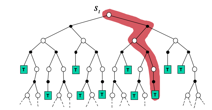
 Backup tree with value iteration based on the MC approach. MC samples a complete trajectory to the terminating node T shown with red. There is some rationale of doing so, if we recall that the state-value function that was defined in the introductory MDP section i.e. the expected return. vπ(s)=Eπ(GtSt=s)v_\pi(s) = \mathop{\mathbb{E}_\pi}(G_t | S_t=s) can be approximated by using the sample mean return over a sample episode / trajectory: Gt(τ)=k=0T1γkRt+1+kG_t(\tau) = \sum_{k=0}^{T-1}\gamma^k R_{t+1+k} The value function is therefore approximated in MC, by the (empirical or sample) mean of the returns over multiple episodes / trajectories. In other words, to update each element of the state value function:
  1. For each time step tt that state ss is visited in an episode
    • Increment a counter N(s)N(s) that counts the visitations of the state ss
    • Calculate the total return GT(s)=GT(s)+GtG^T(s) = G^T(s) + G_t
  2. At the end of multiple episodes, the value is estimated as V(s)=GT(s)/N(s)V(s) = G^T(s) / N(s)
As N(s)N(s) \rightarrow ∞ the estimate will converge to V(s)vπ(s)V(s) \rightarrow v_\pi(s). But we can also do the following trick, called incremental mean approximation: μk=1kj=1kxj=1k(xk+j=1k1xj) \mu_k = \frac{1}{k} \sum_{j=1}^k x_j = \frac{1}{k} \left( x_k + \sum_{j=1}^{k-1} x_j \right) =1k(xk+(k1)μk1))=μk1+1k(xkμk1) = \frac{1}{k} \left(x_k + (k-1) \mu_{k-1}) \right) = \mu_{k-1} + \frac{1}{k} ( x_k - \mu_{k-1} ) Using the incremental sample mean, we can approximate the value function after each episode if for each state ss with return GtG_t, N(s)=N(s)+1N(s) = N(s) +1 V(s)=V(s)+α(GtV(s)) V(s) = V(s) + \alpha \left( G_t - V(s) \right) where α=1N(s)\alpha = \frac{1}{N(s)} can be interpreted as a forgetting factor. α\alpha can also be any number <1< 1 to get into a more flexible sample mean - the running mean that will increase the robustness of this approach in non-stationary environments. An important fact about Monte Carlo methods is that the estimates for each state are independent. The estimate for one state does not build upon the estimate of any other state, as is the case in DP. In other words, Monte Carlo methods do not bootstrap. In particular, note that the computational expense of estimating the value of a single state is independent of the number of states. This can make Monte Carlo methods particularly attractive when one requires the value of only one or a subset of states. The policy evaluation problem for action values is to estimate qπ(s,a)q_π(s,a), the expected return when starting in state ss, taking action aa, and thereafter following policy ππ. The Monte Carlo methods for this are essentially the same as just presented for state values and in fact the estimated Q(s,a)Q(s,a) function is the only one that allows us to apply model-free control via the a generalized version of the policy iteration algorithm. This is because the policy improvement step for V(s)V(s), does require the knowledge of MDP dynamics while the equivalent step for Q(s,a)Q(s,a) does not.
Connect these docs to Claude, VSCode, and more via MCP for real-time answers.