

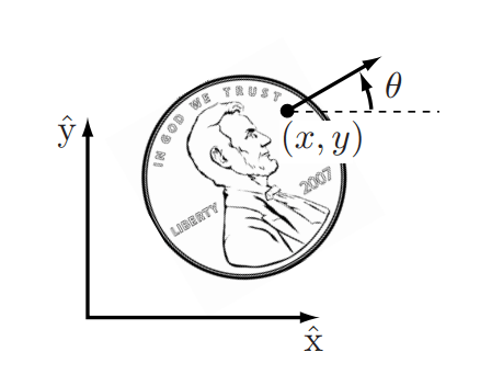
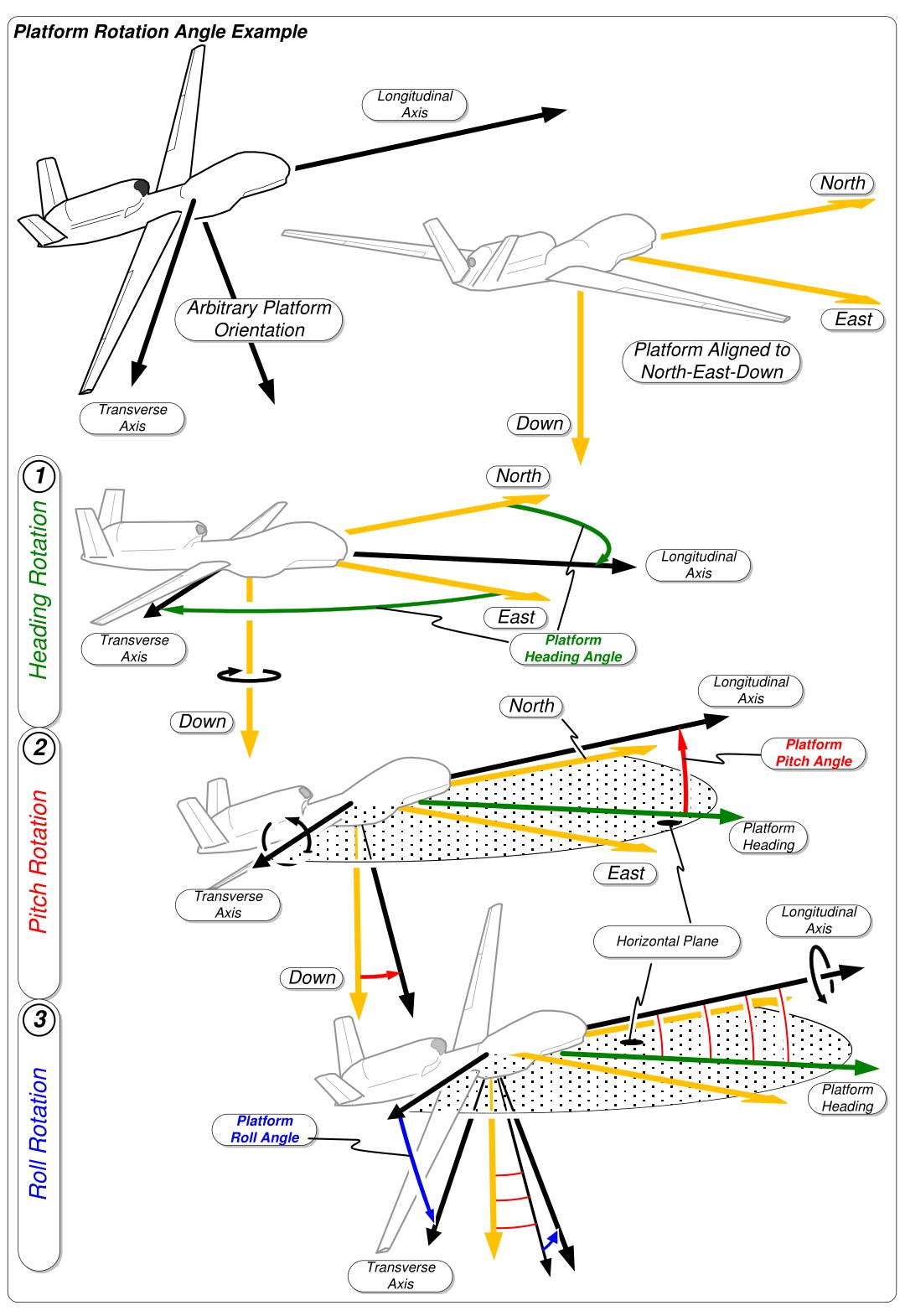
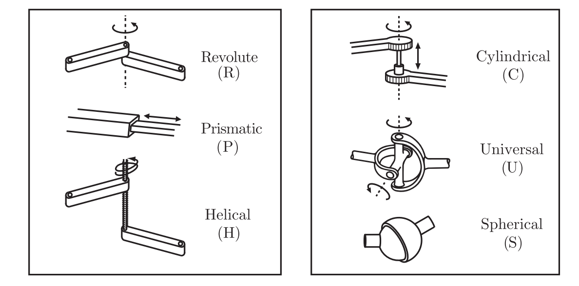
This section borrows heavily from chapter 2, Configuration Space, of Kevin Lynch and Frank Park, Modern Robotics: Mechanics, Planning, and Control (Cambridge University Press, 2017). You can download the chapter as a PDF. A robot is mechanically constructed by connecting a set of bodies, called links,to each other using various types of joints.Actuators, such as electric motors,deliver forces or torques that cause the robot’s links to move. Usually an end-effector, such as a gripper or hand for grasping and manipulating objects, is attached to a specific link. A robot’s configuration is the specification of the positions of all points of the robot’s mechanisms. We start by presenting the configuration of simple objects such as a coin shown lying heads up on a table. We call such objects planar rigid bodies to distinguish them from spatial rigid bodies that can be anywhere in the 3D space. The coin’s configuration, can be described by three real numbers (also called coordinates): two coordinates (x,y)(x,y) specify the location of a particular point on the coin, and one coordinate (θθ) specifies the coin’s orientation. If the coin may also lie tails up, the face showing is part of its configuration too, but it takes values in the discrete set {heads,tails}\{\text{heads}, \text{tails}\} rather than in a continuous range of real numbers. Configuration of a coin on a flat surface. The fact that I can freely place the coin anywhere on a table, affords two degress of freedom. One for each of the (x,y)(x,y) coordinates of the point on the coin. The point itself however is not enough to fix its configuration: if for example the point is the eye of the Abraham Lincoln, we have an additional degree of freedom - he can look anywhere (360 deg) and this is captured via the angle θ\theta. The number of degrees of freedom (dof) of a robot, is the smallest number of real-valued coordinates needed to represent its configuration. The discrete face therefore adds no degree of freedom. The coin lying on a table has f=3f=3 three degrees of freedom and its current configuration is a point in the space containing all possible configurations of the robot, called the configuration space (C-space). As another example, a large drone when considering it as a single rigid body for navigation purposes only, has 6-DoF - three angles and three cartesian coordinates, as shown. Heading, pitch and roll rotations of an aircraft relative to a North-East-Down reference frame Pitch, yaw (heading), and roll around the principal axis of an drone located at point p=(x,y,z)T\mathbf p = (x,y,z)^T. Figure by the Motion Imagery Standards Board, public domain. One important point to keep in mind: in the drone example we used one of the many configuration representation possibilities - there are many more and each one of them has its advantages and disadvantages. In addition the drone has 6-dof if considered a single rigid body (fuselage) and we ask a question as to its configuration for navigation purposes. When we ask other questions though such as its kinematics and dynamics we no longer can treat it as single rigid body as there are tens of links and joints that right now we dont consider (eg. flaps) that effect its kinematic and dynamic behavior. Therefore, for a robot in general we talk about many rigid bodies that come together and each one is constrained from the overall mechanical structure of the robot. In general the dof of a robot are given by dof=(freedoms of the bodies)−(independent constraints)\mathrm{dof} = \text{(freedoms of the bodies)} - \text{(independent constraints)} Lets see now how joints constrain the motion of any rigid body and reduce the overall degrees of freedom. The revolute joint (R), also called a hinge joint, allows rotational motion about the joint axis. From everyday life a door has three revolute joints. The prismatic joint (P), also called a sliding or linear joint, allows translational (or rectilinear) motion along the direction of the joint axis. A sliding door is a good analogy to think about. The helical joint (H), also called a screw joint, allows simultaneous rotation and translation about a screw axis. Revolute, prismatic, and helical joints all have one degree of freedom. Joints can also have multiple degrees of freedom. The cylindrical joint (C) has two degrees of freedom and allows independent translations and rotations about a single fixed joint axis. The universal joint (U) is another two-degreeof-freedom joint that consists of a pair of revolute joints arranged so that their joint axes are orthogonal. The spherical joint (S), also called a ball-and-socket joint, has three degrees of freedom and functions much like our shoulder joint. The following table captures the dof of each joint in the case where the joint connects planar and spatial rigid bodies. There is a formula that provides the degrees of freedom of a robot, known as Grubler’s rule: dof=m(N−1−J)+∑i=1Jfi\mathrm{dof} = m \left( N - 1 - J \right) + \sum_{i=1}^{J} f_i where m=3m = 3 for planar mechanisms and m=6m = 6 for spatial mechanisms, NN is the number of links (including the ground link), JJ is the number of joints, and fif_i is the number of degrees of freedom of joint ii. The formula assumes the constraints enforced by the joints are independent. If they are not, as can happen in closed chains, it gives only a lower bound on the number of degrees of freedom.

How many dof does the human arm have?
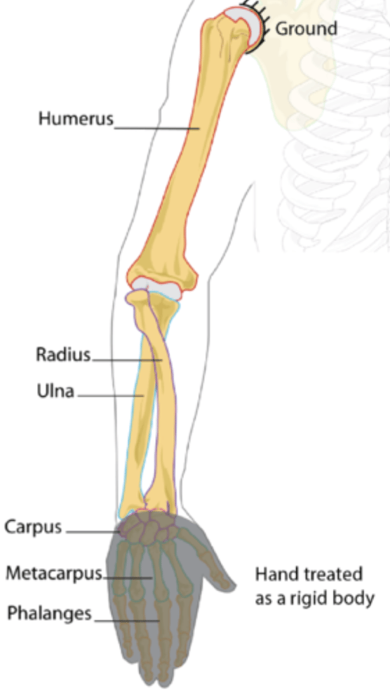
Human arm.Count from your torso to your palm, keeping the center of your shoulder stationary and leaving the fingers out. Each joint of the arm is one of the types listed above:The links are the torso, the upper arm, the forearm and the palm, so N=4N = 4 and J=3J = 3. Grubler’s rule givesdof=6(N−1−J)+∑i=1Jfi=6(4−1−3)+7=7\mathrm{dof} = 6 \left( N - 1 - J \right) + \sum_{i=1}^{J} f_i = 6 \left( 4 - 1 - 3 \right) + 7 = 7

Configuration space topology

Consider a point moving on the surface of a sphere. The point’s C-space is two dimensional, as the configuration can be described by two coordinates, latitude and longitude. As another example, a point moving on a flat surface (a plane) also has a two-dimensional C-space, with coordinates (x, y). While both a plane and the surface of a sphere are two dimensional, clearly they do not have the same shape: the plane extends infinitely while the sphere wraps around. An oval-shaped American football also wraps around similarly to a sphere. The only difference between a football and a sphere is that the football has been stretched in one direction. The idea that the two-dimensional surfaces of a small sphere, a large sphere, and a football all have the same kind of shape, which is different from the shape of a plane, is expressed by the topology of the surfaces. Example topologies are shown in the figure. Examples of C-space topologies. For example, S2S^2 is the two-dimensional surface of a sphere in three-dimensional space. The configuration space (C-space) of a rigid body in the plane can be written as R2×S1\mathbb{R}^2 \times S^1, since the configuration can be represented as the concatenation of the coordinates (x,y)(x, y), which form R2\mathbb{R}^2, and an angle θ\theta, which forms S1S^1. The configuration space (C-space) of a 2R robot arm can be written as S1×S1=T2S^1 \times S^1 = T^2, where TnT^n is the nn-dimensional surface of a torus in an (n+1)(n+1)-dimensional space. Note that S1×S1×⋯×S1S^1 \times S^1 \times \cdots \times S^1 (with nn copies of S1S^1) is equal to TnT^n, not SnS^n; for example, a sphere S2S^2 is not topologically equivalent to a torus T2T^2. Note that the topology of a space is a fundamental property of the space itself and is independent of how we choose coordinates to represent points in the space.For example, to represent a point on a circle, we could refer to the point by the angle θ from the center of the circle to the point, relative to a chosen zero angle. Or, we could choose a reference frame with its origin at the center of the circle and represent the point by the two coordinates (x, y) subject to the constraint x2+y2=1x^2 + y^2 = 1. No matter what our choice of coordinates is, the space itself does not change.
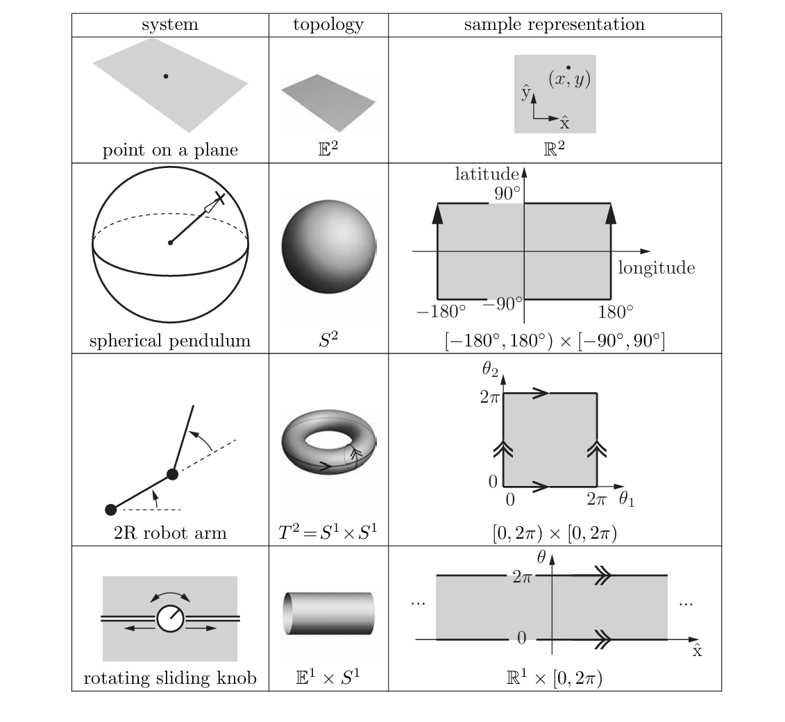
C-space Representation

Consider the topological space of a sphere as an example. One solution for a sphere is to use latitude and longitude coordinates.
In general a choice of nn coordinates, or parameters, to represent an n-dimensional space is called an explicit parametrization of the topology of the space.
A point on the spherical surface can be represented like the well understood coordinates we use for earth navigation:
  • Latitude (ϕ): angle from the equator (−90° at South Pole to +90° at North Pole)
  • Longitude (λ): angle around the equator (from −180° to +180°)
This coordinate system works well almost everywhere, except at the poles. Imagine you’re very close to the North Pole (ϕ ≈ 90°), and you take a tiny step eastward. Your latitude ϕ barely changes (still near 90°) but your longitude λ may change a lot, even flip from +180° to −180° with just a tiny move. This means that small physical motions lead to large changes in the coordinates, a situation that is called a singularity that is not a flaw of the sphere itself (which is smooth and uniform), but a limitation of the chosen representation. These singularities especially cause problems when computing velocities, because coordinate rates (like ϕ˙\dot\phi, λ˙\dot\lambda) can become very large or even diverge near the poles, despite the actual speed in 3D space being constant. The video is illustrative of such issues.
To avoid such singularities, we use an implicit representation instead of an explicit parametrization. An implicit representation views the nn-dimensional space as embedded in a Euclidean space of more than nn dimensions, just as a two-dimensional unit sphere can be viewed as a surface embedded in three-dimensional Euclidean space. An implicit representation uses the coordinates of the higher-dimensional space (for example, (x,y,z)(x, y, z) in three-dimensional space), but subjects these coordinates to constraints that reduce the number of degrees of freedom. For the unit sphere, the constraint equation is: x2+y2+z2=1x^2 + y^2 + z^2 = 1 A disadvantage of this approach is that the representation involves more variables than the actual number of degrees of freedom, however as it turns out it offers the ability to perform linear operations and therefore its not necessarily computationally inefficient. As we will see the implicit representation afforded by rotation matrices, encode orientation in 3D space, uses nine numbers subject to three constraints and is a linear operator.

Task space

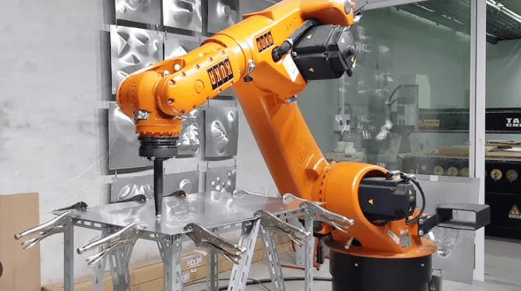
The task space is a space in which the robot’s task can be naturally expressed. Consider incremental sheet forming, shown below. A metal sheet is clamped in a frame and the robot pushes a tool with a spherical tip into it, following a path that gradually forms the part. The formed surface is determined by the path of the center of the tip, and rotating the tool about that center does not change it. The task space is then R3\mathbb{R}^3, the position (x,y,z)(x, y, z) of the tip. If the part is formed in layers of constant depth, each layer is a contour in a plane and the task space of a layer is R2\mathbb{R}^2. If the tool has to be tilted, for example so that its shank does not hit the wall of a deep part, the direction of the tool becomes part of the task and the task space is R3×S2\mathbb{R}^3 \times S^2. The task space is a choice made when describing the task and does not depend on the robot. A 6-dof arm performing a task in R3\mathbb{R}^3 has three degrees of freedom left over, which can be used for other purposes such as staying away from singularities or from the clamping frame. A robot arm pressing a tool into a clamped metal sheet. Incremental sheet forming.
Workspace

The workspace is a specification of the configurations that the end-effector of the robot can reach. The definition of the workspace is primarily driven by the robot’s structure, independently of the task.

References

Lynch and Park, Modern Robotics: Mechanics, Planning, and Control (2017)