Pinhole Camera Model

​

Introduction to Camera Models

The camera models are mathematical representations of how a camera captures the 3D world and projects it onto a 2D image plane. There are several different camera models, each with its own assumptions and characteristics. Some of the most common camera models include:

1. Pinhole Camera Model: This is the simplest camera model, which assumes that light rays pass through a single point (the pinhole) and project onto the image plane. It is characterized by its focal length and the position of the pinhole.
2. Perspective Camera Model: This model extends the pinhole camera model by incorporating lens distortion and other optical effects. It is commonly used in computer vision and graphics to simulate realistic camera behavior.
3. Orthographic Camera Model: In this model, parallel lines in the 3D world remain parallel in the 2D image. This is useful for technical drawings and architectural visualizations, where accurate measurements are important.
4. Spherical Camera Model: This model captures a 360-degree view of the scene by using a spherical image sensor. It is commonly used in virtual reality and panoramic photography.
5. Omnidirectional Camera Model: Similar to the spherical camera model, this model captures a wide field of view (FOV) by using multiple lenses or a fisheye lens. It is often used in robotics and surveillance applications.

Each of these camera models has its own set of equations and parameters that describe how 3D points are projected onto the 2D image plane. Understanding these models is essential for tasks such as image rectification, 3D reconstruction, and camera calibration. Here we focus on the pinhole camera model. Pinhole camera model. The image is formed on the image plane by light rays passing through a small aperture (the pinhole) at the center of projection. The image is inverted and smaller than the object.

​

Camera Model Fundamentals

​

Pinhole Camera Model

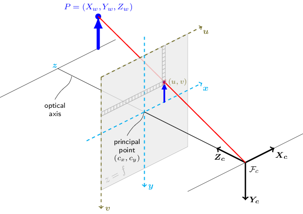
The functions in this section use a so-called pinhole camera model. The view of a scene is obtained by projecting a scene’s 3D point $P_w$ into the image plane using a perspective transformation which forms the corresponding pixel $p$. Both $P_w$ and $p$ are represented in homogeneous coordinates, i.e. as 3D and 2D homogeneous vector respectively. The distortion-free projective transformation given by a pinhole camera model is: $\lambda \; p = K \begin{bmatrix} R|t \end{bmatrix} P_w$ where:

• $P_w$ is a 3D point expressed with respect to the world coordinate system
• $p$ is a 2D pixel in the image plane
• $K$ is the camera intrinsic matrix
• $R$ and $t$ are the rotation and translation that describe the change of coordinates from world to camera coordinate systems
• $\lambda$ is the projective transformation’s arbitrary scaling

​

Camera Intrinsic Matrix

The camera intrinsic matrix $K$ projects 3D points given in the camera coordinate system to 2D pixel coordinates: $p = K P_c$ The camera intrinsic matrix $K$ is composed of the focal lengths $f_x$ and $f_y$, which are expressed in pixel units, and the principal point $(c_x, c_y)$, that is usually close to the image center: $K = \begin{bmatrix} f_x & 0 & c_x \\ 0 & f_y & c_y \\ 0 & 0 & 1 \end{bmatrix}$ and thus: $\lambda \begin{bmatrix} u \\ v \\ 1 \end{bmatrix} = \begin{bmatrix} f_x & 0 & c_x \\ 0 & f_y & c_y \\ 0 & 0 & 1 \end{bmatrix} \begin{bmatrix} X_c \\ Y_c \\ Z_c \end{bmatrix}$

​

Coordinate Transformations

The joint rotation-translation matrix $[R|t]$ is the matrix product of a projective transformation and a homogeneous transformation. The 3-by-4 projective transformation maps 3D points represented in camera coordinates to 2D points in the image plane and represented in normalized camera coordinates $x' = X_c / Z_c$ and $y' = Y_c / Z_c$. The homogeneous transformation is encoded by the extrinsic parameters $R$ and $t$ and represents the change of basis from world coordinate system $w$ to the camera coordinate system $c$: $P_c = \begin{bmatrix} R & t \\ 0 & 1 \end{bmatrix} P_w$ This gives us the complete transformation: $\lambda \begin{bmatrix} u \\ v \\ 1 \end{bmatrix} = \begin{bmatrix} f_x & 0 & c_x \\ 0 & f_y & c_y \\ 0 & 0 & 1 \end{bmatrix} \begin{bmatrix} r_{11} & r_{12} & r_{13} & t_x \\ r_{21} & r_{22} & r_{23} & t_y \\ r_{31} & r_{32} & r_{33} & t_z \end{bmatrix} \begin{bmatrix} X_w \\ Y_w \\ Z_w \\ 1 \end{bmatrix}$ If $Z_c \neq 0$, this is equivalent to: $\begin{bmatrix} u \\ v \end{bmatrix} = \begin{bmatrix} f_x X_c/Z_c + c_x \\ f_y Y_c/Z_c + c_y \end{bmatrix}$

​

Lens Distortion Model

Real lenses introduce distortions (radial and tangential).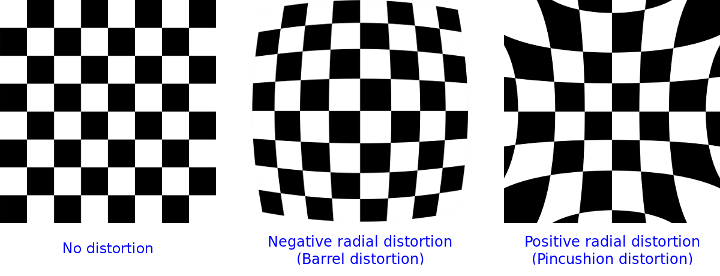 Distortion examples: barrel, pincushion, and tangential distortions. The extended camera model accounts for this: $\begin{bmatrix} u \\ v \end{bmatrix} = \begin{bmatrix} f_x x'' + c_x \\ f_y y'' + c_y \end{bmatrix}$ where: $\begin{bmatrix} x'' \\ y'' \end{bmatrix} = \begin{bmatrix} x' \frac{1 + k_1 r^2 + k_2 r^4 + k_3 r^6}{1 + k_4 r^2 + k_5 r^4 + k_6 r^6} + 2 p_1 x' y' + p_2(r^2 + 2 x'^2) + s_1 r^2 + s_2 r^4 \\ y' \frac{1 + k_1 r^2 + k_2 r^4 + k_3 r^6}{1 + k_4 r^2 + k_5 r^4 + k_6 r^6} + p_1 (r^2 + 2 y'^2) + 2 p_2 x' y' + s_3 r^2 + s_4 r^4 \end{bmatrix}$ with $r^2 = x'^2 + y'^2$ and $\begin{bmatrix} x' \\ y' \end{bmatrix} = \begin{bmatrix} X_c/Z_c \\ Y_c/Z_c \end{bmatrix}$ if $Z_c \neq 0$. Distortion Parameters:

• Radial coefficients: $k_1$, $k_2$, $k_3$, $k_4$, $k_5$, $k_6$
• Tangential coefficients: $p_1$, $p_2$
• Thin prism coefficients: $s_1$, $s_2$, $s_3$, $s_4$

The distortion coefficients are passed as: $(k_1, k_2, p_1, p_2[, k_3[, k_4, k_5, k_6 [, s_1, s_2, s_3, s_4[, \tau_x, \tau_y]]]])$ Types of Distortion:

• Barrel distortion: $(1 + k_1 r^2 + k_2 r^4 + k_3 r^6)$ monotonically decreasing
• Pincushion distortion: $(1 + k_1 r^2 + k_2 r^4 + k_3 r^6)$ monotonically increasing

​

Coordinate Systems

​

Right-handed vs Left-handed

The right-handed and left-handed coordinate systems are two conventions for defining the orientation of axes in 3D space.

​

ROS2 Coordinate System

The table below shows what ROS2 RViz2 displays - it’s a right-handed coordinate system. The right-hand rule is used to determine the direction of the axes.

​

Sensor Coordinate Systems

Each sensor has its own coordinate system, supported by the vendor documentation, which may be right-handed or left-handed. Take for example RealSense cameras - a right-handed sensor.

---

References

- Mur-Artal, R., Tardos, J. (2016). ORB-SLAM2: an Open-Source SLAM System for Monocular, Stereo and RGB-D Cameras.
- Tatarchenko, M., Dosovitskiy, A., Brox, T. (2015). Multi-view 3D Models from Single Images with a Convolutional Network.