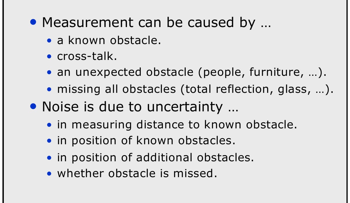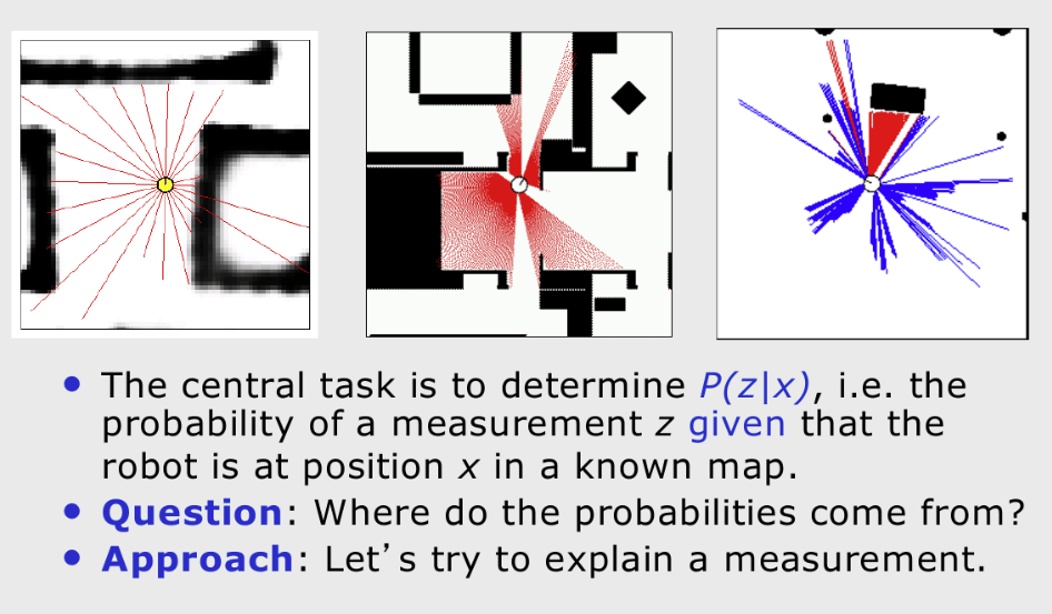
Beam-based Sensor Models

Beam-based distance sensors (sonar, lidar, depth IR) measure the distance to the nearest surface along discrete directions called beams. This section develops a probabilistic forward (generative) model $p(\mathbf z_t \mid \mathbf x_t, m)$ for the likelihood of receiving a range scan $\mathbf z_t$ from pose $\mathbf x_t$ in map $m$. It also develops an inverse model for occupancy mapping. Notation:

• Robot pose (planar): $\mathbf x_t = (x_t, y_t, \theta_t)$.
• Map $m$: an occupancy grid (binary or probabilistic) or a geometric representation (polygonal or mesh).
• Scan: $\mathbf z_t = { z_t^k }_{k=1}^K$ with beam angles $\phi_k$ relative to sensor frame.
• Maximum sensor range: $z_{\max}$.
• Expected (ideal) range along beam $k$: $\hat z_t^k = r(\mathbf x_t, \phi_k, m)$ found via ray casting.

We approximate the beams as conditionally independent: $$p(\mathbf z_t \mid \mathbf x_t, m) = \prod_{k=1}^K p(z_t^k \mid \mathbf x_t, m).$$

​

Beam-based forward model

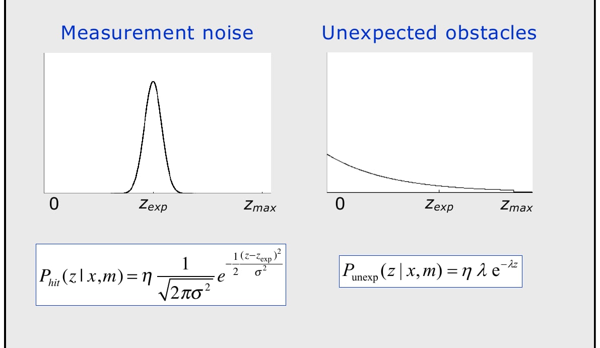
Real measurements include precise hits, unexpected short returns, max-range readings (no return), and random noise. We model each beam with a weighted mixture: $$p(z \mid \hat z) = \alpha_{\text{hit}} p_{\text{hit}}(z \mid \hat z) + \alpha_{\text{short}} p_{\text{short}}(z \mid \hat z) + \alpha_{\text{max}} p_{\text{max}}(z) + \alpha_{\text{rand}} p_{\text{rand}}(z),$$ with $\sum_i \alpha_i = 1$.

​

Precise hit component

$$p_{\text{hit}}(z \mid \hat z) = \begin{cases} \eta \exp\!\left(-\dfrac{(z - \hat z)^2}{2\sigma_{\text{hit}}^2}\right), & 0 \le z \le z_{\max}\\ 0, & \text{otherwise} \end{cases}$$ $\eta$ normalizes over $[0,z_{\max}]$.

​

Unexpected short return

This component represents unmodeled obstacles between the sensor and the predicted surface: $$p_{\text{short}}(z \mid \hat z) = \begin{cases} \eta \lambda e^{-\lambda z}, & 0 \le z \le \hat z\\ 0, & z > \hat z \end{cases}$$

​

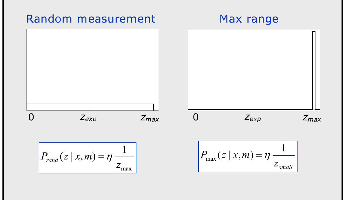
Maximum range

$$p_{\text{max}}(z) = \begin{cases} 1, & z = z_{\max}\\ 0, & \text{otherwise} \end{cases}$$

​

Random noise

$$p_{\text{rand}}(z) = \begin{cases} \dfrac{1}{z_{\max}}, & 0 \le z < z_{\max}\\ 0, & \text{otherwise} \end{cases}$$

​

Per-beam likelihood

$$p(z_t^k \mid \mathbf x_t, m) = p(z \mid \hat z_t^k).$$ For numerical stability, use the log likelihood: $$\log p(\mathbf z_t \mid \mathbf x_t, m) = \sum_k \log\left( \sum_j \alpha_j p_j(z_t^k) \right).$$

​

Parameter estimation

Given a training set ${ (z_n, \hat z_n)}$:

• If the component assignments are known, estimate $\sigma_{\text{hit}}^2$ in closed form from the weighted residual variance.
• Otherwise, use expectation-maximization (EM):
  • In the E-step, compute the responsibilities $r_{ni} = \dfrac{\alpha_i p_i(z_n)}{\sum_j \alpha_j p_j(z_n)}$.
  • In the M-step, set $\alpha_i = \frac{1}{N}\sum_n r_{ni}$ and update $\sigma_{\text{hit}}, \lambda$ by weighted maximum likelihood estimation.

Constrain the mixture weights so that $\alpha_i \ge 0$, $\sum\alpha_i=1$.

​

Dynamic obstacles

Add a dynamic layer $m_D$ to the forward model: $$p(z \mid \hat z, m, m_D) = (1-\beta) p(z \mid \hat z, m) + \beta p_{\text{dyn}}(z),$$ where $p_{\text{dyn}}$ can assign more probability to short or random returns. Motion segmentation determines $\beta$. Key references: (Zeng et al., 2016)

​

References

• Zeng, A., Song, S., Nießner, M., Fisher, M., Xiao, J., et al. (2016). 3DMatch: Learning Local Geometric Descriptors from RGB-D Reconstructions. arXiv [cs.CV].

---