Homogeneous Coordinates

Under perspective projection, the parallel tracks appear to meet at a point on the horizon. A photograph maps points from three-dimensional Euclidean space to a two-dimensional image plane. This perspective projection does not preserve circles, distances, angles, or ratios of distances. For example, a circle can appear as an ellipse. Straight lines remain straight, while parallel lines can appear to meet. A projective space extends Euclidean space so that every pair of lines intersects. Parallel lines intersect at a point at infinity. Choosing coordinates selects an origin, but any point could serve as the origin.

A point expressed in two different coordinate frames.

The coordinates of a point in 2D depend on the chosen coordinate system. The solid and dashed axes define two coordinate systems, so the same point has different coordinates in each. Its position in space does not change. The figure shows two frames. Each frame consists of an origin and two linearly independent basis vectors that define the axes of the two-dimensional space. More generally, an origin

p_o

and

n

linearly independent basis vectors define an n-dimensional affine frame. For any vector

\mathbf v

, there is a unique set of scalars

s_i

such that

\mathbf v = s_1 \mathbf u_1 + s_2 \mathbf u_2 + ... + s_n \mathbf u_n = \mathbf s^T [\mathbf u_1, \mathbf u_2, ..., \mathbf u_n]^T

where

\mathbf s

gives the coordinates of

\mathbf v

in the frame. Each point also has unique scalars

s_i

that express it in terms of the origin

p_o

and the basis vectors:

p = p_o + s_1 \mathbf u_1 + s_2 \mathbf u_2 + ... + s_n \mathbf u_n = p_o + \mathbf s^T [\mathbf u_1, \mathbf u_2, ..., \mathbf u_n]^T

An affine space of dimension

n

consists of a set of points

\mathcal{A}

and an associated vector space

V

of dimension

n

. It supports two operations:

Point subtraction: $p - q \in V$ (gives a vector)
Point translation: $p + v \in \mathcal{A}$ (moves a point by a vector)

There is no fixed origin, no preferred coordinate system, and no basis until you choose one.A coordinate frame on an affine space is a chosen origin point

p_0 \in \mathcal{A}

and a basis

\{v_1, \dots, v_n\}

for the associated vector space

V

.A vector space has a built-in origin, defined by the zero vector. It is closed under addition and scalar multiplication, so it supports linear combinations such as

a\mathbf{v}_1 + b\mathbf{v}_2

. For this reason, it is also called a linear space. In an affine space, you cannot add two points directly, and there is no zero point.Euclidean space adds an inner product, which defines angles and lengths.

Points and vectors may both have x, y, and z coordinates in 3D, but they are different mathematical objects. A 3D frame defined by

(p_o, \mathbf u_1, \mathbf u_2, \mathbf u_3)

does not by itself distinguish a point

(p_x, p_y, p_z)

from a vector

(v_x, v_y, v_z)

with the same coordinates. Homogeneous coordinates resolve this ambiguity. In this frame, the point is

p = [s_1 s_2 s_3 1][\mathbf u_1 \mathbf u_2 \mathbf u_3 p_o]^T

and the vector is

\mathbf v = [s_1' s_2' s_3' 0][\mathbf u_1 \mathbf u_2 \mathbf u_3 p_o]^T

The point representation

[s_1 s_2 s_3 1]

and the vector representation

[s_1' s_2' s_3' 0]

are called homogeneous coordinates. The fourth coordinate

w

is called the weight. A point

(x,y,z)

in three-dimensional Euclidean space can be represented by the 4-tuple

(x,y,z,1)

. More generally,

(x,y,z,1)

and

(\lambda x, \lambda y, \lambda z, \lambda)

represent the same point for any

\lambda \neq 0

, because dividing every coordinate by

\lambda

gives

(x,y,z,1)

. A point with weight

w \neq 0

therefore stands for the Cartesian point obtained by dividing through by the weight:

(x, y, z, w) \equiv (x/w,\; y/w,\; z/w), \qquad w \neq 0

Homogeneous coordinates represent a family of equivalent points along a ray in projective space. Each member is a scaled version of the same Cartesian point. These coordinates can:

Represent points at infinity (when $w = 0$ ), as required for parallel lines in perspective projections.
Express transformations such as perspective camera models and 3D projections as linear matrix operations.

Transformations in homogeneous coordinates

This section gives homogeneous matrix representations for common 2D transformations.

Rigid transformation

A rigid transformation consists of a rotation and a translation. It preserves lengths and angles and does not include scaling or shearing. Its matrix is:

\mathbf{T}_{\text{rigid}} = \begin{bmatrix} \cos\theta & -\sin\theta & t_x \\ \sin\theta & \cos\theta & t_y \\ 0 & 0 & 1 \end{bmatrix}

$\theta$ : rotation angle
$(t_x, t_y)$ : translation

Similarity transformation

A similarity transformation includes rotation, translation, and uniform scaling. It preserves shape but not necessarily size.

\mathbf{T}_{\text{sim}} = \begin{bmatrix} s \cos\theta & -s \sin\theta & t_x \\ s \sin\theta & s \cos\theta & t_y \\ 0 & 0 & 1 \end{bmatrix}

Here,

s

is the scaling factor.

Affine transformation

An affine transformation can combine translation, rotation, scaling, and shearing. It preserves parallel lines, but it need not preserve lengths or angles.

\mathbf{T}_{\text{affine}} = \begin{bmatrix} a_{11} & a_{12} & t_x \\ a_{21} & a_{22} & t_y \\ 0 & 0 & 1 \end{bmatrix}

This is the general form of a 2D affine transformation.

Example

The following code applies these transformations to a square:

import matplotlib.pyplot as plt
import numpy as np

# Original square: corner at origin, size 1
square = np.array(
    [
        [0, 0, 1],
        [1, 0, 1],
        [1, 1, 1],
        [0, 1, 1],
        [0, 0, 1],  # close the square
    ]
).T


# Define transformations
def apply_transform(matrix, shape):
    return (matrix @ shape).T[:, :2]


# Rigid: rotate 45 deg and translate (1, 1)
theta = np.pi / 4
T_rigid = np.array(
    [[np.cos(theta), -np.sin(theta), 1], [np.sin(theta), np.cos(theta), 1], [0, 0, 1]]
)

# Similarity: scale by 1.5, rotate 30 deg, translate (0.5, 0.5)
theta_sim = np.pi / 6
s = 1.5
T_similarity = np.array(
    [
        [s * np.cos(theta_sim), -s * np.sin(theta_sim), 0.5],
        [s * np.sin(theta_sim), s * np.cos(theta_sim), 0.5],
        [0, 0, 1],
    ]
)

# Affine: shear and scale
T_affine = np.array([[1.2, 0.5, 1.5], [0.2, 1.0, 1.0], [0, 0, 1]])

# Translation only
T_translation = np.array([[1, 0, 2], [0, 1, 1], [0, 0, 1]])

# Apply transformations
square_rigid = apply_transform(T_rigid, square)
square_similarity = apply_transform(T_similarity, square)
square_affine = apply_transform(T_affine, square)
square_translation = apply_transform(T_translation, square)
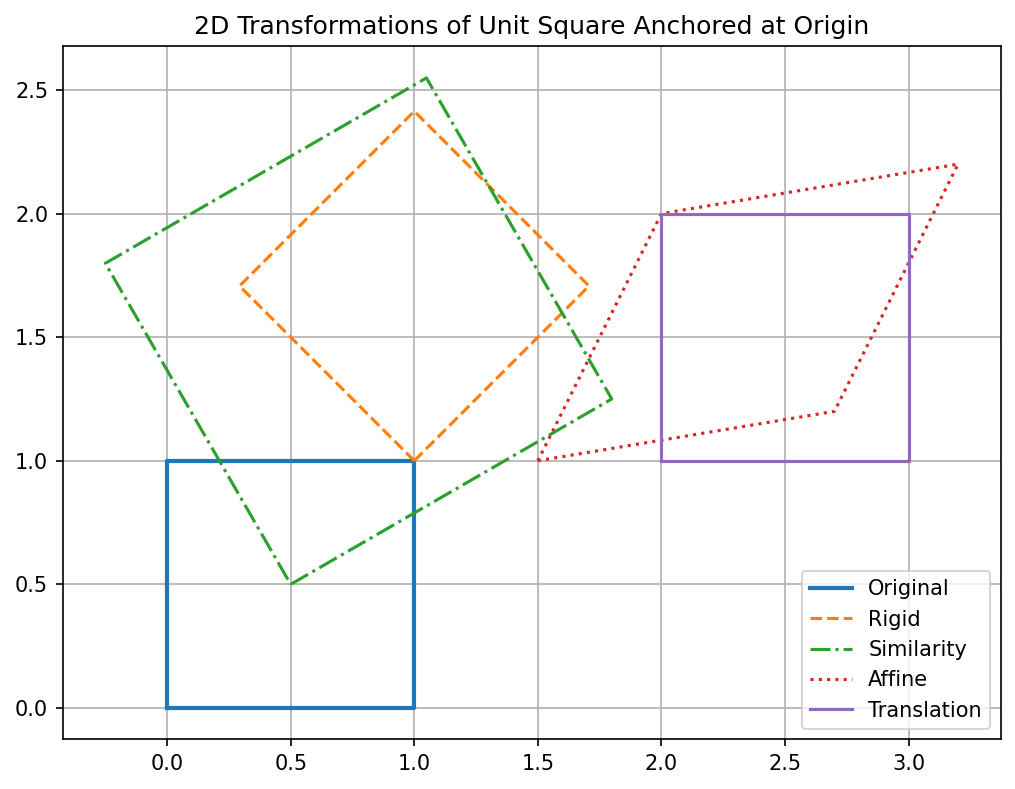
square_original = square.T[:, :2]

Key references: (Zeng et al., 2016; Chang et al., 2017; Qi et al., 2016; Bronstein et al., 2016; Mur-Artal & Tardos, 2016)

References

Bronstein, M., Bruna, J., LeCun, Y., Szlam, A., Vandergheynst, P. (2016). Geometric deep learning: going beyond Euclidean data.
Chang, A., Dai, A., Funkhouser, T., Halber, M., Nießner, M., et al. (2017). Matterport3D: Learning from RGB-D Data in Indoor Environments.
Mur-Artal, R., Tardos, J. (2016). ORB-SLAM2: an Open-Source SLAM System for Monocular, Stereo and RGB-D Cameras.
Qi, C., Su, H., Mo, K., Guibas, L. (2016). PointNet: Deep Learning on Point Sets for 3D Classification and Segmentation.
Zeng, A., Song, S., Nießner, M., Fisher, M., Xiao, J., et al. (2016). 3DMatch: Learning Local Geometric Descriptors from RGB-D Reconstructions.

Edit this page on GitHub or file an issue.

Robotics Systems

Kinematics & Dynamics

Sensor Models

Systems Integration

Homogeneous Coordinates

Transformations in homogeneous coordinates

Rigid transformation

Similarity transformation

Affine transformation

Example

References

​Transformations in homogeneous coordinates

​Rigid transformation

​Similarity transformation

​Affine transformation

​Example

​References

Transformations in homogeneous coordinates

Rigid transformation

Similarity transformation

Affine transformation

Example

References