Rigid-body Motions

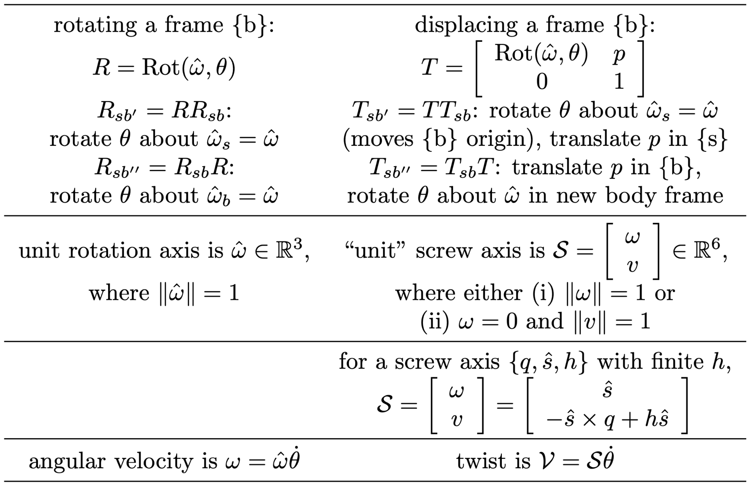
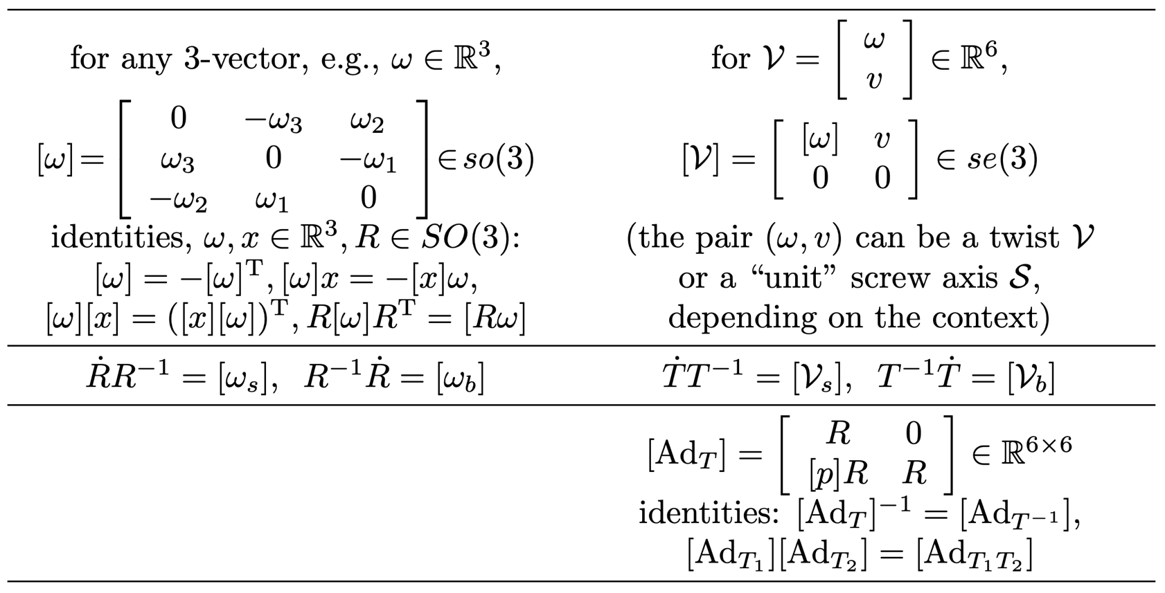
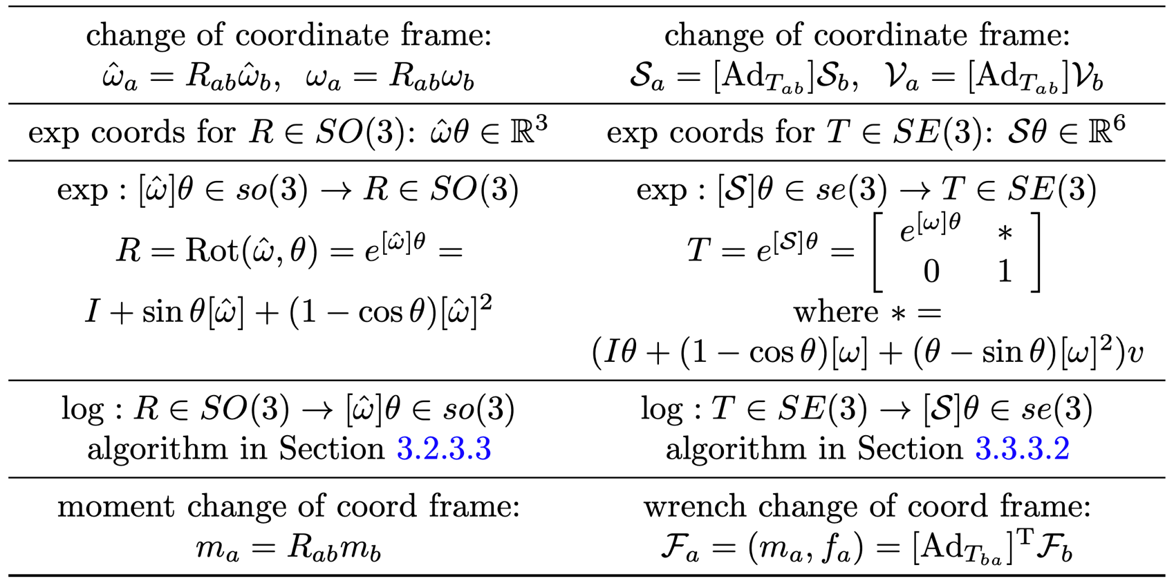
This section borrows heavily from chapter 3, Rigid-Body Motions, of Kevin Lynch and Frank Park, Modern Robotics: Mechanics, Planning, and Control (Cambridge University Press, 2017). You can download the chapter as a PDF. Robotics uses several motion representations for different modeling needs. These include rotation matrices, axis-angle representations, quaternions, Euler angles, and other conventions. The choice of representation depends on the application, vendor, and software tools. Aeronautics and self-driving cars may use different conventions because of the robots involved or the history of each field. Robot vendors may also define their own conventions, as in this explanation of robot orientation. Software tools may use other conventions, so system integration may require conversion between representations. Rigid-body motion in three-dimensional space requires an understanding of both position and orientation. A point in space is described by three coordinates, but a rigid body has six degrees of freedom: three for position and three for orientation. Rigid-body configurations are encoded by 4×4 homogeneous transformation matrices. Rotation matrices $R \in SO(3)$ represent orientation. Six-dimensional twists describe spatial velocities. Six-dimensional wrenches represent spatial forces.

​

Vectors and Reference Frames

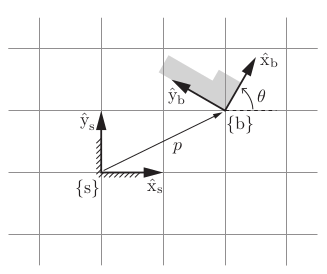
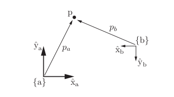
A vector $\mathbf{v} \in \mathbb{R}^n$ is a geometric quantity with magnitude and direction. A vector is independent of coordinates. It acquires numerical values only when expressed in a coordinate frame. For example, a velocity vector may be $\mathbf{v} = [3, 1, 0]^T$ in frame ${a}$ and have different coordinates in frame ${b}$. Points are also represented as vectors. Their coordinates are defined relative to the origin of a reference frame, as shown below. Choose a length scale and a fixed space frame {s}, with unit axes x̂s and ŷs, as shown above. Attach a reference frame with unit axes x̂b and ŷb to the planar body. This frame moves with the body, so it is called the body frame and is denoted {b}. All frames discussed here are inertial. The term “body frame” refers to the inertial frame that instantaneously coincides with the moving frame.

​

Planar Rigid-Body Motions

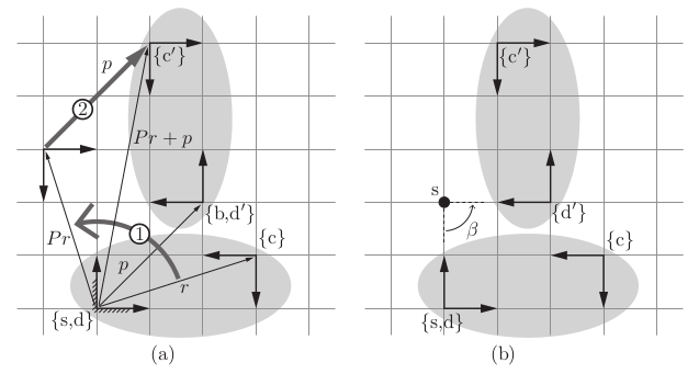
In the plane, a rotation matrix $P \in SO(2)$ and a translation vector $\mathbf{p} \in \mathbb{R}^2$ describe a rigid-body configuration. The pair $(P, \mathbf{p})$ represents a body in the space frame. It also changes the frame used to represent vectors and displaces a point or frame by rotation and translation. For example, consider a point $q$ at $[1, 1]^T$ in a frame that is rotated 60° counterclockwise and translated by $[2, 1]^T$, as shown below. In the fixed frame, the transformation is given by: $$P = \begin{bmatrix} \cos\theta & -\sin\theta \\ \sin\theta & \cos\theta \end{bmatrix}, \quad q' = Pq + \mathbf{p}$$ Although P contains four numbers, three constraints apply. Each column of P must be a unit vector, and the columns must be orthogonal. The remaining degree of freedom is parametrized by θ. The pair (P, p) describes the orientation and position of \{b\} relative to \{s\}. Any planar motion can also be interpreted as a rotation about a fixed point $\mathbf{s}$. The figure below shows such a motion. (a) The frame \{d\} is fixed to an elliptical rigid body and initially coincides with \{s\}. A rotation by P followed by a translation by p displaces it to \{d0\}, which coincides with the stationary frame \{b\}. The pair (P, p) represents \{b\} in \{s\}. The same transformation takes the frame \{c\}, also attached to the rigid body, to \{c0\}. Transformation 1 rotates \{c\} about the origin of \{s\}. Transformation 2 then translates the frame by p expressed in \{s\}. (b) The rotation and translation can also occur simultaneously. In this view, the displacement is a rotation of β = 90° about a fixed point s. This is a planar example of a screw motion. The three screw coordinates $(β, s_x , s_y )$ parametrize the displacement. Here, $(s_x , s_y ) = (0, 2)$ gives the coordinates of point s, which is the screw axis out of the page, in the fixed frame \{s\}.

​

Rotations and Angular Velocities in 3D

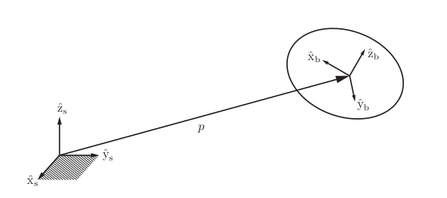
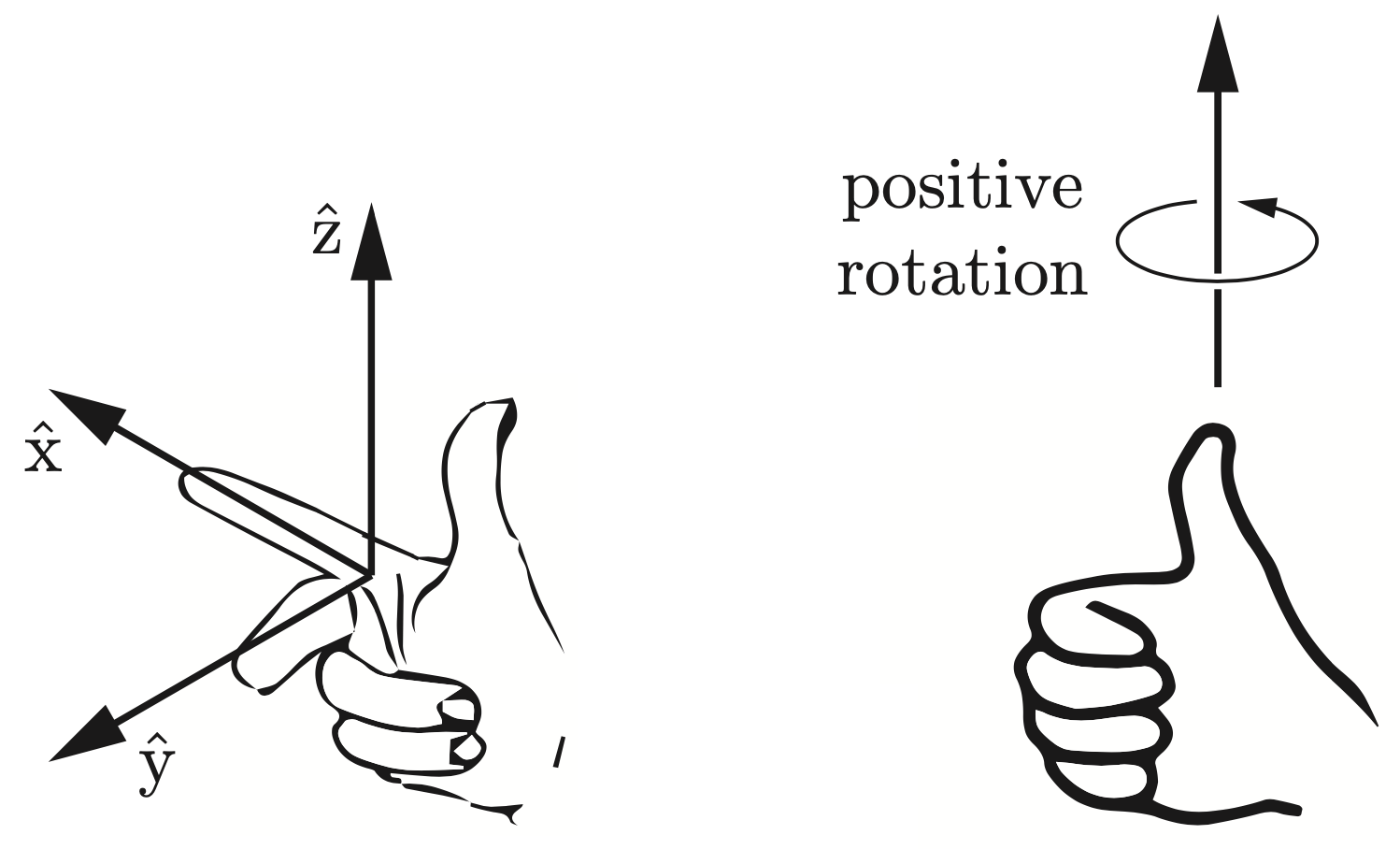
We now consider the general three-dimensional case shown below. All coordinate systems are right-handed. The unit axes follow the right-hand rule and satisfy $\hat x \times \hat y = \hat z$. Let $\mathbf{p}$ denote the vector from the fixed-frame origin to the body-frame origin. In terms of the fixed-frame coordinates, $\mathbf{p}$ can be expressed as: $$\mathbf{p} = p_1 \, \hat{\mathbf{x}}_s + p_2 \, \hat{\mathbf{y}}_s + p_3 \, \hat{\mathbf{z}}_s \tag{3.12}$$ The axes of the body frame can also be expressed in the fixed frame as: $$\hat{\mathbf{x}}_b = r_{11} \hat{\mathbf{x}}_s + r_{21} \hat{\mathbf{y}}_s + r_{31} \hat{\mathbf{z}}_s$$ $$\hat{\mathbf{y}}_b = r_{12} \hat{\mathbf{x}}_s + r_{22} \hat{\mathbf{y}}_s + r_{32} \hat{\mathbf{z}}_s$$ $$\hat{\mathbf{z}}_b = r_{13} \hat{\mathbf{x}}_s + r_{23} \hat{\mathbf{y}}_s + r_{33} \hat{\mathbf{z}}_s$$ We now define the position vector $\mathbf{p} \in \mathbb{R}^3$ and the rotation matrix $R \in \mathbb{R}^{3 \times 3}$ as follows: $$\mathbf{p} = \begin{bmatrix} p_1 \\\\ p_2 \\\\ p_3 \end{bmatrix} \tag{3.13}$$ $$R = \begin{bmatrix} r_{11} & r_{12} & r_{13} \\\\ r_{21} & r_{22} & r_{23} \\\\ r_{31} & r_{32} & r_{33} \end{bmatrix} = \left[ \hat{\mathbf{x}}_b \quad \hat{\mathbf{y}}_b \quad \hat{\mathbf{z}}_b \right] \tag{3.14–3.16}$$ The 12 parameters given by the pair $(R, \mathbf{p})$ provide a complete description of the position and orientation of the rigid body relative to the fixed frame. The special orthogonal group $SO(3)$, also known as the group of rotation matrices, is the set of all $3 \times 3$ real matrices $R$ that satisfy the following properties: $$R^T R = I \quad \text{and} \quad \det R = 1$$ Rotation matrices satisfy $R^{-1} = R^T$. Their product is also a rotation matrix ($R_1 R_2 \in SO(3)$), and they preserve vector lengths ($\|Rv\| = \|v\|$). They represent orientation, change coordinates, and rotate vectors. SO(3) is a curved three-dimensional space. The possible velocities at any point of SO(3) form a flat three-dimensional vector space called the tangent space.

​

Angular Velocities

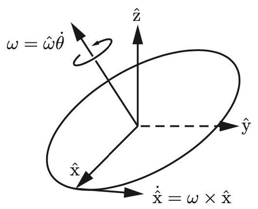
Suppose a frame with unit axes ${\hat{x}, \hat{y}, \hat{z}}$ is attached to a rotating body. Consider the time derivatives of these unit axes. The length of $\hat{x}$ is fixed, so only its direction can change with time. The same holds for $\hat{y}$ and $\hat{z}$. Between times $t$ and $t + \Delta t$, a rotation through an angle $\Delta \theta$ about a unit axis $\hat{\mathbf \omega}$ through the origin describes the change in orientation. The axis $\hat{w}$ is independent of coordinates and has not yet been represented in a reference frame. In the limit as $\Delta t$ approaches zero, the ratio $\Delta \theta / \Delta t$ becomes the rate of rotation $\dot{\theta}$, and $\hat{w}$ can similarly be regarded as the instantaneous axis of rotation. As shown above, $\hat{\mathbf \omega}$ and $\dot{\theta}$ define the angular velocity $\mathbf{\omega}$: $$\mathbf{\omega} = \hat{\mathbf \omega} \, \dot{\theta}$$ Let $R(t)$ be the rotation matrix that describes the orientation of the body frame relative to the fixed frame at time $t$. Its time derivative is $\dot{R}(t)$. The first column of $R(t)$, denoted $\mathbf{r}_1(t)$, gives $\hat{x}$ in fixed-frame coordinates. The columns $\mathbf{r}_2(t)$ and $\mathbf{r}_3(t)$ give $\hat{y}$ and $\hat{z}$ in fixed-frame coordinates. Therefore, $\dot r_i = \mathbf \omega_s \times r_i$ where $i=1,2,3$. It follows that $\dot R = \mathbf \omega_s \times R$ We can replace the cross product with matrix multiplication. Write $\boldsymbol{\omega}_s \times R$ as $[\boldsymbol{\omega}_s] R$, where $[\boldsymbol{\omega}_s]$ is the $3 \times 3$ skew-symmetric matrix representation of $\boldsymbol{\omega}_s \in \mathbb{R}^3$. Page 78 of Lynch and Park derives the angular velocity from rotation matrices. Given $R(t)$, the spatial angular velocity is $[\omega_s] = R \dot{R}^T$ and the body angular velocity is $[\omega_b] = R^T \dot{R}$. The skew-symmetric matrix $[\omega]$ satisfies $[\omega]^T = -[\omega]^T$. The fixed-frame angular velocity $\boldsymbol{\omega}_s$ does not depend on the choice of body frame. Similarly, the body-frame angular velocity $\boldsymbol{\omega}_b$ does not depend on the choice of fixed frame. The equations may appear to depend on both frames because $R$ and $\dot{R}$ each depend on ${s}$ and ${b}$. However, the product $\dot{R} R^{-1}$ is independent of ${b}$, and the product $R^{-1} \dot{R}$ is independent of ${s}$.

​

Exponential Coordinate Representation of Rotations

Rodrigues’ formula provides a way to compute rotation matrices: $$R = I + \sin\theta [\omega] + (1 - \cos\theta)[\omega]^2$$ This formula defines the exponential coordinates of rotation. Any rotation can be expressed as: $$R = e^{[\omega]\theta}$$ The logarithm of a rotation is the inverse of the matrix exponential. If $\theta \neq 0$, then: $$[\omega] = \frac{1}{2 \sin \theta}(R - R^T)$$

​

Rigid-Body Motions in SE(3)

Rigid-body motions in three-dimensional space are described using homogeneous transformation matrices: $$T = \begin{bmatrix} R & \mathbf{p} \\ 0 & 1 \end{bmatrix} \in SE(3)$$ This matrix encodes both rotation and translation. The inverse of a homogeneous transformation matrix is given by: $$T^{-1} = \begin{bmatrix} R^T & -R^T \mathbf{p} \\ 0 & 1 \end{bmatrix}$$ Transformations compose by matrix multiplication: $$T_{ac} = T_{ab} T_{bc}$$

​

Twists (Spatial Velocities)

A twist is a six-dimensional vector that combines angular and linear velocity: $$V = \begin{bmatrix} \omega \\ v \end{bmatrix} \in \mathbb{R}^6$$ The matrix representation of a twist is: $$[V] = \begin{bmatrix} [\omega] & v \\ 0 & 0 \end{bmatrix} \in \mathfrak{se}(3)$$ Body and spatial twists are defined as follows: $[V_b] = T^{-1} \dot{T}$ and $[V_s] = \dot{T} T^{-1}$. The adjoint operator is given by: $$\text{Ad}_T = \begin{bmatrix} R & 0 \\ [\mathbf{p}]R & R \end{bmatrix}, \quad V_s = \text{Ad}_T V_b$$

​

Exponential Coordinates for Rigid Motions

Exponential coordinates provide a compact description of rigid motions. Let $S = (\omega, v) \in \mathbb{R}^6$ be a screw axis. The transformation is: $$e^{[S]\theta} = \begin{bmatrix} e^{[\omega]\theta} & G(\theta)v \\ 0 & 1 \end{bmatrix}$$ where $$G(\theta) = I\theta + (1 - \cos\theta)[\omega] + (\theta - \sin\theta)[\omega]^2$$ Given a transformation $T = (R, \mathbf{p})$, the matrix logarithm is used as follows: $\log R \rightarrow [\omega]\theta$ $v = G(\theta)^{-1} \mathbf{p}$ Thus, $[S]\theta = \log T$.

​

Wrenches (Spatial Forces)

A wrench is a six-dimensional vector that combines force and torque: $$F = \begin{bmatrix} \tau \\ f \end{bmatrix}$$ Here, $f$ is the force and $\tau = r \times f$ is the torque (moment). Coordinate transformations for wrenches are given by: $$F_b = \text{Ad}_T^T F_a$$

​

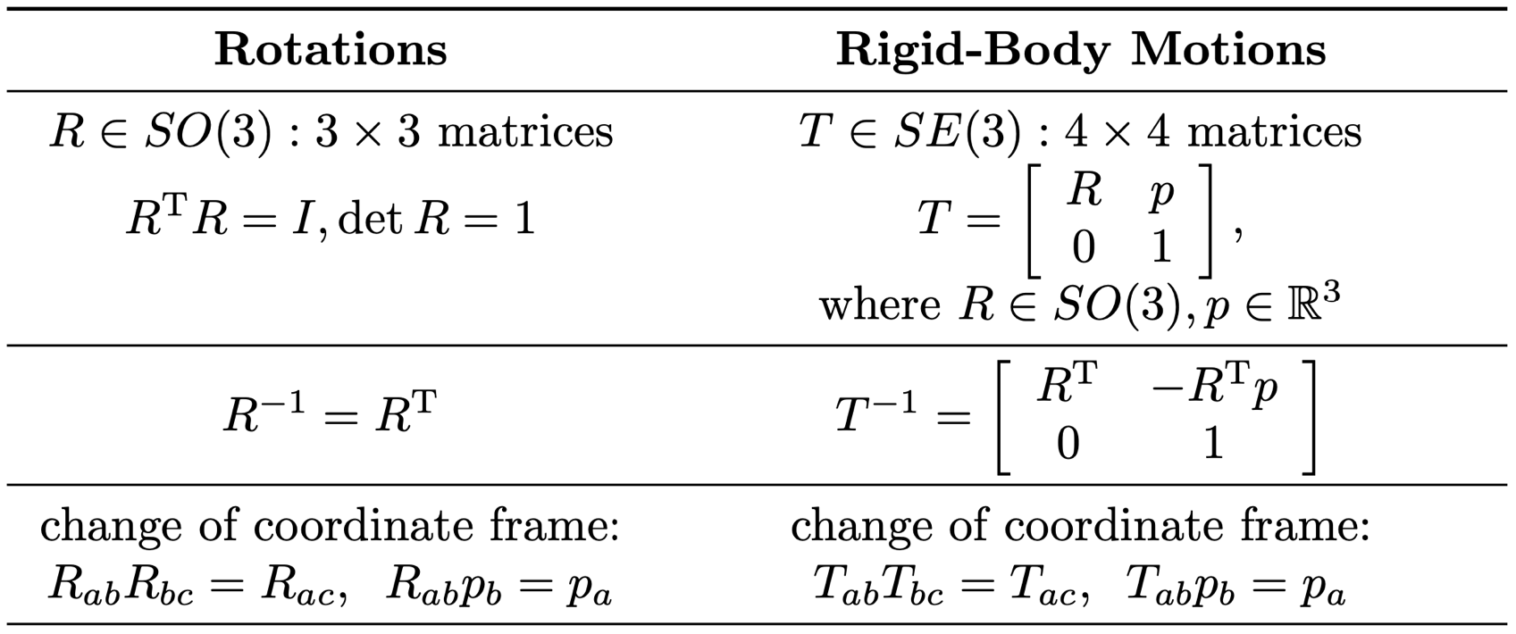
Summary of rotation and motion representations

​

Other representations

​

Euler Angles

Three values are sufficient to describe orientation. Orthogonality and unit vector length impose six constraints on the nine entries of a rotation matrix. An orientation can therefore be represented by rotations through specified angles about the $x$, $y$, and $z$ axes of the reference coordinate system. This representation is called X-Y-Z fixed-angle notation. Its rotation matrix has the form: ^s_BR_{XYZ}(\gamma,\beta,\alpha)=\begin{bsmallmatrix}\cos\alpha & -\sin\alpha & 0\\ \sin\alpha & \cos\alpha & 0\\0 & 0 & 1\end{bsmallmatrix}\begin{bsmallmatrix}cos\beta& 0 & \sin\beta\\0 & 1 & 0\\-\sin\beta & 0 & \cos\beta\end{bsmallmatrix}\begin{bsmallmatrix}1 & 0 & 0 \\ 0 & \cos\gamma & -\sin\gamma\\0 & \sin\gamma & \cos\gamma\end{bsmallmatrix} X-Y-Z fixed angles express a coordinate frame using rotations relative to the original frame ${A}$. Another description starts with a frame ${B}$ that coincides with ${A}$. It then rotates about the Z-axis by $\alpha$, the Y-axis by $\beta$, and the X-axis by $\gamma$. This representation is called Z-Y-X Euler angles. The coordinate axes need not all be different, so there are twelve valid sequences of rotations: XYX, XZX, YXY, YZY, ZXZ, ZYZ, XYZ, XZY, YZX, YXZ, ZXY, and ZYX. Consecutive rotations about the same axis are excluded because they are equivalent to one rotation through the sum of the two angles. No single convention is correct for every application. Hardware and software manufacturers use different conventions, often based on the fields for which their products were developed, such as aviation or geology. These representations have singularities at certain angle values. At such a value, a sequence can be equivalent to consecutive rotations about the same axis. For example, this occurs for the XYZ rotation matrix when the angle about the Y-axis is 90°. Other representations avoid these singularities over the full range of possible motions.

​

Quaternions

Quaternions are often preferred for computational efficiency and numerical stability. A quaternion is a 4-tuple that extends the complex numbers. It has many applications in mathematics, including the representation of orientation and rotation. A quaternion has the form $q=a+b\mathbf{i}+c\mathbf{j}+d\mathbf{k}$ Here, $a$ is the scalar part of the quaternion. The elements $b$, $c$, and $d$ form the vector part. The conjugate of a quaternion is $q^*=a-b\mathbf{i}-c\mathbf{j}-d\mathbf{k}$ Each rotation can be represented by an angle and a single axis in space, called the Euler axis. Given an axis $\hat{K}=[k_x k_y k_z]^T$ and an angle $\theta$, the Euler parameters, or unit quaternion, $\mathbf{q}=(\epsilon_1,\epsilon_2,\epsilon_3,\epsilon_4)$ are \epsilon_1&=\cos \frac{\theta}{2}\\ \epsilon_2&=k_x \sin \frac{\theta}{2}\\ \epsilon_3&=k_y \sin \frac{\theta}{2}\\ \epsilon_4&=k_z \sin\frac{\theta}{2} \end\{align\}$$ These four quantities are constrained by the relationship $$\epsilon_1^2+\epsilon_2^2+\epsilon_3^2+\epsilon_4^2=1$$ This constraint places the quaternion on a unit hypersphere. Given a vector $\mathbf{p} \in \mathbb{R}^3$ and a unit quaternion $\mathbf{q}$, the rotated vector $\mathbf{p'}$ is $$\mathbf{p'}=\mathbf{q}\mathbf{p}\mathbf{q^*}$$ where $\mathbf{q^*}$ is the conjugate of $\mathbf{q}$. The product of two quaternions gives the rotation equivalent to two successive rotations. For quaternions $\epsilon$ and $\epsilon'$, the product is defined by the following matrix multiplication: $$\left[\begin{array}{cccc} \epsilon_4 & \epsilon_1 & \epsilon_2 & \epsilon_3\\ -\epsilon_1 & \epsilon_4 & -\epsilon_3 & \epsilon_2\\ -\epsilon_2 & \epsilon_3 & \epsilon_4 & -\epsilon_1\\ -\epsilon_3 & -\epsilon_2 & \epsilon_1 & \epsilon_4 \end{array}\right] \left[\begin\{array\}\{c\}\epsilon_4'\\\epsilon_1'\\\epsilon_2'\\\epsilon_3'\end\{array\}\right]$$ Multiplying two rotation matrices requires 27 multiplications and 18 additions. Multiplying two quaternions requires 16 multiplications and 12 additions. Quaternions also avoid singularities at specific joint angles. These singularities can have significant effects on physical robots. ## References Lynch and Park, *Modern Robotics: Mechanics, Planning, and Control* (2017) [http://modernrobotics.org](http://modernrobotics.org) --- <Callout icon="pen-to-square" iconType="regular"> [Edit this page on GitHub](https://github.com/aegean-ai/eaia/edit/main/src/aiml-common/lectures/kinematics/motion-representations/index.mdx) or [file an issue](https://github.com/aegean-ai/eaia/issues/new/choose). </Callout>