Open In Colab
import torch
import numpy as np
import matplotlib.pyplot as plt

torch.manual_seed(0)

# Standard normal CDF (used for the dead-ReLU fraction); torch.erf avoids a scipy dependency
def Phi(t):
    t = torch.as_tensor(t, dtype=torch.float32)
    return 0.5 * (1.0 + torch.erf(t / 2.0 ** 0.5))

The gradient of a neuron is proportional to its input

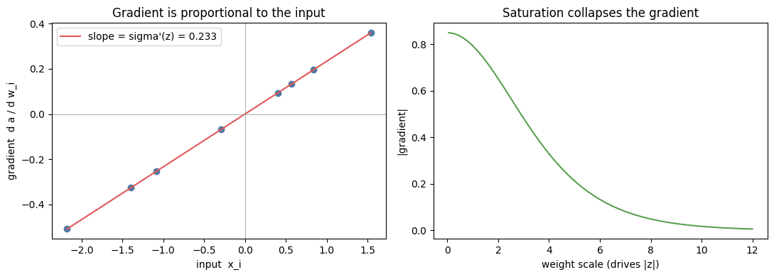
Start with a single neuron. It forms a weighted sum of its inputs and passes it through a sigmoid: z=iwixi+b,a=σ(z)=11+ez.z = \sum_i w_i x_i + b, \qquad a = \sigma(z) = \frac{1}{1+e^{-z}}. The partial derivative of the output with respect to a weight is awi=σ(z)xi=a(1a)xi.\frac{\partial a}{\partial w_i} = \sigma'(z)\, x_i = a(1-a)\, x_i . For any scalar loss LL on top, the chain rule gives Lwi=Laσ(z)δ  xi=δxi.\frac{\partial L}{\partial w_i} = \underbrace{\frac{\partial L}{\partial a}\,\sigma'(z)}_{\delta}\; x_i = \delta\, x_i . Two things to read off. The gradient of weight wiw_i is the input xix_i scaled by a single number δ\delta shared across all weights, so the gradient vector points along the input. And δ\delta carries σ(z)=a(1a)\sigma'(z) = a(1-a), which collapses toward zero when z|z| is large: a saturated neuron has a small gradient no matter how large the input is.
# Single neuron: verify d a / d w_i = sigma'(z) * x_i
n = 8
x = torch.randn(n)
w = torch.randn(n, requires_grad=True)
b = torch.zeros(1, requires_grad=True)

z = w @ x + b
a = torch.sigmoid(z)
a.backward()                      # gradient of the scalar output a

sigma_prime = (a * (1 - a)).item()
ratio = w.grad / x                # should be constant = sigma'(z) for every i
print(f"sigma'(z)      = {sigma_prime:.6f}")
print(f"grad_i / x_i   = {ratio.tolist()}")

assert torch.allclose(ratio, torch.full((n,), sigma_prime), atol=1e-5), "grad not proportional to input"
print("OK: gradient is proportional to the input, slope = sigma'(z)")
sigma'(z)      = 0.233472
grad_i / x_i   = [0.2334718108177185, 0.2334717959165573, 0.2334718108177185, 0.2334718108177185, 0.2334717959165573, 0.2334717959165573, 0.2334718108177185, 0.2334718108177185]
OK: gradient is proportional to the input, slope = sigma'(z)
Output from cell 3

Extending to a fully connected ReLU layer

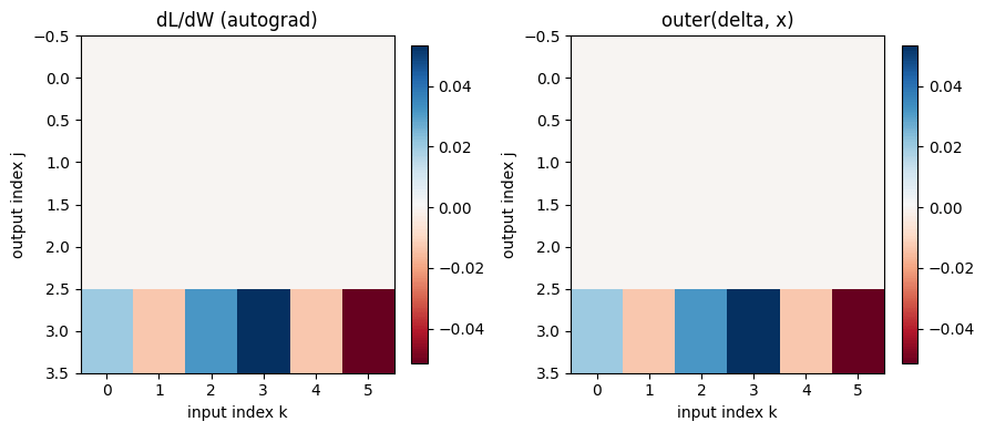
A fully connected layer applies z=Wx+bz = Wx + b and then a ReLU, a=ReLU(z)a = \mathrm{ReLU}(z). ReLU has derivative 1[z>0]\mathbb{1}[z>0], so ajWjk=1[zj>0]xk,ajbj=1[zj>0].\frac{\partial a_j}{\partial W_{jk}} = \mathbb{1}[z_j>0]\, x_k, \qquad \frac{\partial a_j}{\partial b_j} = \mathbb{1}[z_j>0]. With an upstream gradient g=L/ag = \partial L/\partial a and the gate m=1[z>0]m = \mathbb{1}[z>0], write δ=gm\delta = g \odot m. Then LW=δx(an outer product),Lb=δ.\frac{\partial L}{\partial W} = \delta\, x^\top \quad(\text{an outer product}), \qquad \frac{\partial L}{\partial b} = \delta . Every row of L/W\partial L/\partial W is the input vector xx scaled by one entry of δ\delta, so again the weight gradient points along the input. Keep an eye on the bias gradient, L/b=δ\partial L/\partial b = \delta: there is no factor of xx in it. That asymmetry returns later.
# FC + ReLU: verify dL/dW = outer(delta, x) and dL/db = delta
d_in, d_out = 6, 4
x = torch.randn(d_in)
W = torch.randn(d_out, d_in, requires_grad=True)
b = torch.randn(d_out, requires_grad=True)

z = W @ x + b
a = torch.relu(z)
g = torch.randn(d_out)            # arbitrary upstream gradient dL/da
a.backward(g)

m = (z > 0).float()               # ReLU gate
delta = g * m
expected_dW = torch.outer(delta, x)
expected_db = delta

assert torch.allclose(W.grad, expected_dW, atol=1e-6), "dL/dW mismatch"
assert torch.allclose(b.grad, expected_db, atol=1e-6), "dL/db mismatch"
print("OK: dL/dW = outer(delta, x), every row is x scaled; dL/db = delta")
OK: dL/dW = outer(delta, x), every row is x scaled; dL/db = delta
Output from cell 5

Controlling the input distribution with batch normalization

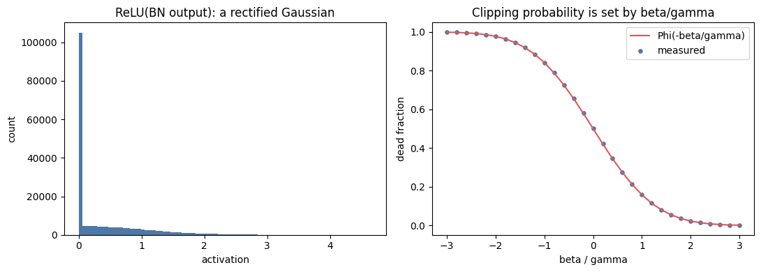
Because each layer’s weight gradient is the input scaled by δ\delta, the scale of the inputs feeding a layer sets the scale of its gradients. Batch normalization standardizes those values per feature across a mini-batch, x^=xμbatchσbatch2+ϵ,x~=γx^+β,\hat{x} = \frac{x - \mu_{\text{batch}}}{\sqrt{\sigma^2_{\text{batch}} + \epsilon}}, \qquad \tilde{x} = \gamma \hat{x} + \beta, with learnable scale γ\gamma and shift β\beta. This is the cheap, per-feature, differentiable relative of whitening: whitening removes all correlations by working with the full covariance matrix, while batch normalization only fixes the per-feature mean and variance (the diagonal). Place batch normalization before the ReLU. If the pre-activation is approximately Gaussian, then x~N(β,γ2)\tilde{x} \sim \mathcal{N}(\beta, \gamma^2) and ReLU(x~)\mathrm{ReLU}(\tilde{x}) is a rectified Gaussian: a spike of zeros plus the positive tail. The fraction of dead units is P(x~0)=Φ ⁣(βγ),P(\tilde{x} \le 0) = \Phi\!\left(-\frac{\beta}{\gamma}\right), so β/γ\beta/\gamma sets how much of the distribution the ReLU clips to zero.
N = 200000
zhat = torch.randn(N)             # BN output before the affine
gamma, beta = 1.0, 0.0
zt = gamma * zhat + beta
out = torch.relu(zt)

dead_measured = (out == 0).float().mean().item()
dead_predicted = Phi(-beta / gamma).item()
print(f"dead fraction measured  = {dead_measured:.4f}")
print(f"dead fraction predicted = Phi(-beta/gamma) = {dead_predicted:.4f}")
assert abs(dead_measured - dead_predicted) < 0.01
dead fraction measured  = 0.5019
dead fraction predicted = Phi(-beta/gamma) = 0.5000
Output from cell 7

Training and inference

Batch normalization behaves differently in the two phases. During training, each mini-batch is normalized with its own mean and variance, so the statistics a sample sees depend on the other samples in the batch. During inference you want the output for a given input to be fixed, so the layer instead uses running estimates of the mean and variance, accumulated as moving averages over the training batches. The learnable scale and shift are applied in both phases.

Where this intuition breaks down

The build above is the story usually told for batch normalization. Most of it is a useful heuristic rather than a theorem. This section keeps the parts that survive scrutiny and shows, with one short experiment each, where the rest fails.

The bias gradient does not scale with the input

The weight gradient carries a factor of xx; the bias gradient, L/b=δ\partial L/\partial b = \delta, does not. Hold the ReLU gate fixed (set b=0b=0 so scaling xx by a positive constant cannot flip any sign) and scale the input. The weight gradient scales with it; the bias gradient does not.
d_in, d_out = 6, 4
# A fixed positive input direction and a fixed weight matrix whose rows give a
# mixed ReLU gate (some units active, some clipped), so the demonstration is
# deterministic regardless of any earlier sampling.
x0 = torch.tensor([1.0, 0.5, 0.8, 0.3, 0.6, 0.9])
W = torch.tensor([
    [ 0.6, -0.2,  0.5, -0.1,  0.3, -0.4],   # active for x0
    [-0.5,  0.1, -0.3,  0.2, -0.6,  0.1],   # clipped
    [ 0.2,  0.4, -0.1,  0.3, -0.2,  0.5],   # active
    [-0.3, -0.2,  0.1, -0.4,  0.2, -0.1],   # clipped
])
g = torch.tensor([1.0, -0.5, 0.8, 0.3])     # arbitrary upstream gradient dL/da

dW_norms, db_norms = [], []
for s in [1.0, 10.0, 100.0]:
    Wv = W.clone().requires_grad_(True)
    bv = torch.zeros(d_out, requires_grad=True)   # b = 0 keeps the gate fixed under positive scaling
    a = torch.relu(Wv @ (x0 * s) + bv)
    a.backward(g)
    dW_norms.append(Wv.grad.norm().item())
    db_norms.append(bv.grad.norm().item())
    print(f"scale={s:6.1f}  |dL/dW|={Wv.grad.norm():9.3f}   |dL/db|={bv.grad.norm():7.4f}")

# Weight gradient grows with the input scale; the bias gradient is invariant to it.
assert dW_norms[0] < dW_norms[1] < dW_norms[2]
assert max(db_norms) - min(db_norms) < 1e-6
print("dL/dW grows with the input scale; dL/db is unchanged.")
scale=   1.0  |dL/dW|=    2.273   |dL/db|= 1.2806
scale=  10.0  |dL/dW|=   22.729   |dL/db|= 1.2806
scale= 100.0  |dL/dW|=  227.288   |dL/db|= 1.2806
dL/dW grows with the input scale; dL/db is unchanged.

Standardizing is not Gaussianizing

Batch normalization fixes only the first two moments. A bimodal pre-activation, standardized, has mean 0\approx 0 and variance 1\approx 1 but is still bimodal: the “clipped Gaussian” picture is a central-limit approximation that becomes accurate only as the layer fan-in grows.
N = 200000
z_bimodal = torch.cat([torch.randn(N // 2) - 3.0, torch.randn(N // 2) + 3.0])
zhat = (z_bimodal - z_bimodal.mean()) / z_bimodal.std()
print(f"after BN: mean={zhat.mean():.4f}, std={zhat.std():.4f} (but shape is still bimodal)")

# CLT: pre-activation = sum of `fan_in` independent contributions; approaches Gaussian as fan_in grows
fan_ins = [1, 2, 8, 64]
clt = {}
for k in fan_ins:
    contrib = (torch.rand(N, k) - 0.5)     # bounded, clearly non-Gaussian summands
    s = contrib.sum(1)
    clt[k] = ((s - s.mean()) / s.std()).numpy()
after BN: mean=0.0000, std=1.0000 (but shape is still bimodal)
Output from cell 10

Batch normalization is not whitening

Per-feature standardization leaves the off-diagonal covariance untouched. Two strongly correlated pre-activations stay correlated after batch normalization, so the per-unit clipping picture ignores how units co-activate. Removing that correlation is exactly what whitening does, at a cost batch normalization avoids.
N = 200000
rho = 0.9
cov = torch.tensor([[1.0, rho], [rho, 1.0]])
L = torch.linalg.cholesky(cov)
z = torch.randn(N, 2) @ L.T

zhat = (z - z.mean(0)) / z.std(0)          # BN: per-feature standardize
corr_after = torch.corrcoef(zhat.T)[0, 1].item()
print(f"input correlation        = {rho}")
print(f"correlation after BN     = {corr_after:.4f}  (essentially unchanged)")
assert abs(corr_after - rho) < 0.02
input correlation        = 0.9
correlation after BN     = 0.9000  (essentially unchanged)

The clipping probability is learned, not enforced

Because γ\gamma and β\beta are trainable, batch normalization does not pin the distribution to N(0,1)\mathcal{N}(0,1). The affine step can reproduce any mean and variance, which means the dead fraction Φ(β/γ)\Phi(-\beta/\gamma) is something the network learns, not something the layer imposes.
zhat = torch.randn(200000)
for gamma, beta in [(1.0, 0.0), (3.0, -2.0), (0.5, 5.0)]:
    y = gamma * zhat + beta
    print(f"gamma={gamma:4.1f}, beta={beta:5.1f} -> mean={y.mean():7.3f}, std={y.std():6.3f}, "
          f"dead=Phi(-beta/gamma)={Phi(-beta/gamma).item():.3f}")
gamma= 1.0, beta=  0.0 -> mean=  0.000, std= 1.002, dead=Phi(-beta/gamma)=0.500
gamma= 3.0, beta= -2.0 -> mean= -1.999, std= 3.006, dead=Phi(-beta/gamma)=0.748
gamma= 0.5, beta=  5.0 -> mean=  5.000, std= 0.501, dead=Phi(-beta/gamma)=0.000

What actually controls the gradient magnitude: scale invariance

The defensible version of “batch normalization controls the gradient” needs no Gaussian assumption. Batch normalization is invariant to the scale of the weights feeding it, BN(aWx)=BN(Wx)\mathrm{BN}(aWx) = \mathrm{BN}(Wx), so the forward pass ignores the weight scale and the gradient absorbs it inversely: L(aW)=1aLW.\frac{\partial L}{\partial (aW)} = \frac{1}{a}\,\frac{\partial L}{\partial W}. Large weights therefore produce proportionally smaller gradients, which decouples the effective step size from the parameter scale.
def bn(u, eps=1e-5):
    return (u - u.mean(0)) / torch.sqrt(u.var(0, unbiased=False) + eps)

# A non-trivial objective: match the normalized output to a fixed target. Its
# gradient is non-zero, so the scale-invariance relation below is meaningful.
x = torch.randn(64, 6)
target = torch.randn(64, 5)
W = torch.randn(6, 5, requires_grad=True)
loss1 = ((bn(x @ W) - target) ** 2).sum(); loss1.backward()
g1 = W.grad.clone()

a = 10.0
Wa = (W.detach() * a).requires_grad_(True)
out2 = bn(x @ Wa)
loss2 = ((out2 - target) ** 2).sum(); loss2.backward()
g2 = Wa.grad.clone()

# The forward pass ignores the weight scale, and the gradient absorbs it inversely.
out_match = torch.allclose(bn(x @ W.detach()), out2, atol=1e-4)
rel_err = ((g2 * a - g1).abs().max() / g1.abs().max()).item()
print(f"BN output scale-invariant: {out_match}")
print(f"gradient 1/a relation, relative error: {rel_err:.1e}")
assert out_match, "BN output should be scale-invariant"
assert rel_err < 1e-3, "gradient should scale as 1/a"
print("OK: BN(aWx) = BN(Wx) and dL/d(aW) = (1/a) dL/dW")
BN output scale-invariant: True
gradient 1/a relation, relative error: 2.3e-05
OK: BN(aWx) = BN(Wx) and dL/d(aW) = (1/a) dL/dW

Why batch normalization actually helps

The motivation in this build, “the gradient depends on the input, so we must control the input distribution”, is the internal covariate shift argument from the original paper. Later work (Santurkar et al., 2018) showed batch normalization does not actually reduce covariate shift: injecting noise after batch normalization, which increases the shift, still trains well. The measured effect is a smoother loss landscape, with more predictive (Lipschitz) gradients, which is what lets you raise the learning rate. The figure below shows the gradient distribution at initialization is far better behaved with batch normalization than without. Histograms of gradients at initialization for a deep layer. With batch normalization the gradients concentrate around the mean; without it the distribution has heavy tails. Gradients at initialization: concentrated with batch normalization (left), heavy-tailed without (right).

What survives

  • The weight gradient really is proportional to the input, for a single neuron and for a fully connected ReLU layer.
  • The bias gradient is not: it depends on the input only through the ReLU gate.
  • “Batch normalization before ReLU controls a clipped Gaussian” is an approximation. It fixes two moments, assumes the rest is Gaussian (true only for wide layers), and leaves correlations in place, so it is not whitening.
  • The clipping probability Φ(β/γ)\Phi(-\beta/\gamma) is learned through the affine parameters, not imposed by the layer.
  • The claim that holds without a Gaussian assumption is scale invariance, BN(aWx)=BN(Wx)\mathrm{BN}(aWx)=\mathrm{BN}(Wx) with gradients scaling as 1/a1/a. The optimization benefit is landscape smoothing, not the removal of internal covariate shift.
  • Whether batch normalization sits before or after the ReLU is an empirical choice, not a theoretical requirement.

References

PyTorch reference

PyTorch classDescription
nn.BatchNorm1dApplies Batch Normalization over a 2D or 3D input.
nn.BatchNorm2dApplies Batch Normalization over a 4D input.
nn.BatchNorm3dApplies Batch Normalization over a 5D input.