L2 Regularization
The most common form of regularization. It penalizes the squared magnitude of all parameters directly in the objective: where is the hidden layer index and is the weight tensor. L2 regularization heavily penalizes peaky weight vectors and prefers diffuse weight vectors. Due to multiplicative interactions between weights and inputs, this encourages the network to use all of its inputs a little rather than some of its inputs a lot.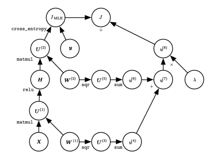
L1 Regularization
For each weight , add the term to the objective. L1 regularization leads weight vectors to become sparse during optimization (exactly zero). Neurons with L1 regularization use only a sparse subset of their most important inputs. Comparison:- L1: Sparse weights, feature selection
- L2: Diffuse small weights, generally better performance
Dropout
An extremely effective regularization technique from Srivastava et al., 2014. During training, dropout keeps a neuron active with probability , or sets it to zero otherwise.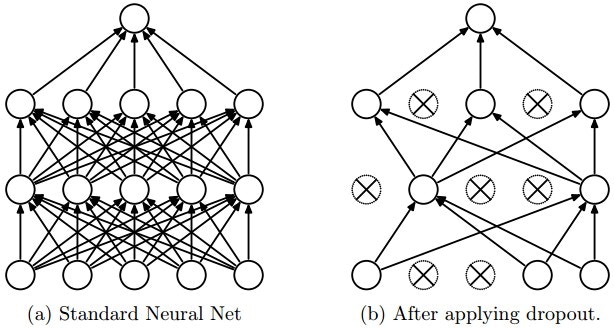
Standard Dropout
Inverted Dropout
Performs scaling at train time, leaving inference untouched:Inverted dropout is preferred because prediction code remains unchanged when tuning dropout placement or probability.
Early Stopping
Monitors validation loss during training and stops when validation error increases, retrieving the best model. This acts as an implicit L2 regularizer: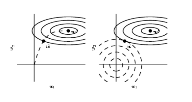
Practical Recommendations
- Use a single, global L2 regularization strength (cross-validated)
- Apply Dropout after all layers (default , tune on validation)
- Combine with Batch Normalization (note: interesting interference between the two)
- Use Early Stopping with patience parameter
References
- Srivastava et al., 2014 - Dropout: A Simple Way to Prevent Neural Networks from Overfitting
- Wan et al., 2013 - Regularization of Neural Networks using DropConnect
- Li et al., 2018 - Understanding the Disharmony between Dropout and Batch Normalization
PyTorch reference
| PyTorch class | Description |
|---|---|
nn.Dropout | During training, randomly zeroes some of the elements of the input tensor with probability . |
nn.Dropout2d | Randomly zero out entire channels. |