Principal Component Analysis (PCA)

Comprehensive PCA tutorial covering dimensionality reduction, noise filtering, and eigenfaces

Introduction

Consider an artificial data set constructed by taking one of the off-line digits, represented by a 64 x 64 pixel grey-level image, and embedding it in a larger image of size 100 x 100 by padding with pixels having the value zero (corresponding to white pixels) in which the location and orientation of the digit is varied at random, as illustrated in the figure below.

manifold-number-three — A synthetic data set obtained by taking one of the off-line digit images and creating multiple copies in each of which the digit has undergone a random displacement and rotation within some larger image field. The resulting images each have 100 x 100 = 10,000 pixels.

Each of the resulting images is represented by a point in the 100 x 100 = 10,000-dimensional data space. However, across a data set of such images, there are only three degrees of freedom of variability, corresponding to the vertical and horizontal translations and the rotations. The data points will therefore live on a subspace of the data space whose intrinsic dimensionality is three.

For real digit image data, there will be a further degree of freedom arising from scaling. Moreover there will be multiple additional degrees of freedom associated with more complex deformations due to the variability in an individual’s writing as well as the differences in writing styles between individuals.

Geometric interpretation

Can we define PCA from a graphical point of view? This is shown in the next figure.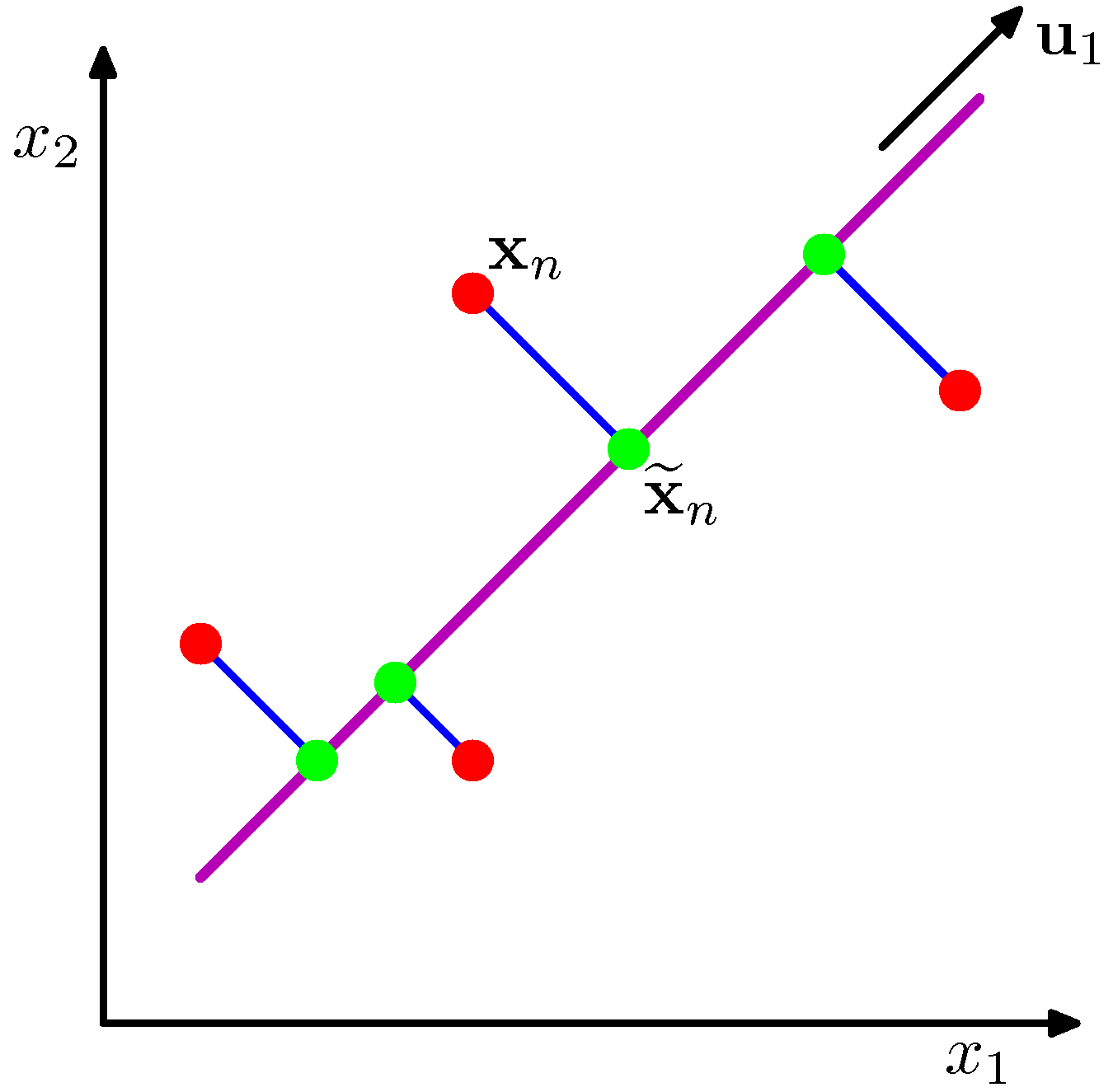

principal-subspace — PCA seeks a space of lower dimensionality (the magenta line) such that the orthogonal projection of the data points into the subspace maximizes the variance of the projected points (green dots) or equivalently minimizes the squared distances of the projection errors (blue lines).

Key concepts

PCA is fundamentally a dimensionality reduction algorithm, but it can also be useful as a tool for:

Visualization - Project high-dimensional data to 2D or 3D for plotting

Noise filtering - Reconstruct data using only the largest principal components

Feature extraction - Discover the most important directions of variance

Data compression - Represent data with fewer dimensions while preserving information

Applications covered in this chapter

Introducing PCA - Principal axes and explained variance

PCA as dimensionality reduction - Projecting to lower dimensions

PCA for visualization - Hand-written digits example

Choosing the number of components - Explained variance ratio

PCA as noise filtering - Denoising images

Eigenfaces - Face recognition with PCA

Foundations

Learning & Regression

Optimization

Maximum Likelihood

Classification

Dimensionality Reduction

Principal Component Analysis (PCA)

PCA Workshop

3D PCA Visualization

Introduction

Geometric interpretation

Key concepts

Applications covered in this chapter

References

PCA Workshop

3D PCA Visualization

​Introduction

​Geometric interpretation

​Key concepts

​Applications covered in this chapter

​References

Introduction

Geometric interpretation

Key concepts

Applications covered in this chapter

References