Visualizing MLE with a Gaussian
To visualize the above, let’s start with a simple Gaussian distribution.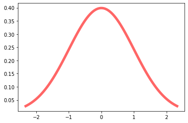
Comparing Hypotheses
Assume now that someone is giving us an array of values and ask us to estimate a that is a ‘good fit’ to the given data. How can we go about solving this problem with Maximum Likelihood Estimation (MLE)? Notice that probability and likelihood have a reverse relationship. Probability attaches to possible results; likelihood attaches to hypotheses. The likelihood function gives the relative likelihoods of different values for the parameter(s) of the distribution from which the data are assumed to have been drawn, given those data.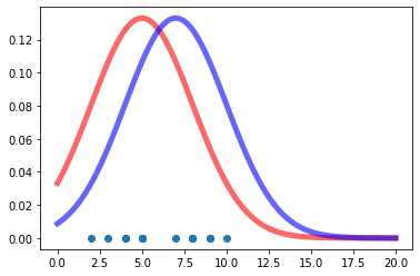
Computing Log-Likelihood
It’s important to safeguard against underflow that may result from multiplying many numbers (for large datasets) that are less than 1.0 (probabilities). So we do the calculations in the log domain using the identity: Let’s look at a function that calculates the log-likelihood for two hypotheses given the data:Searching the Parameter Space
We can search the hypothesis space (parameter space) for the best parameter set :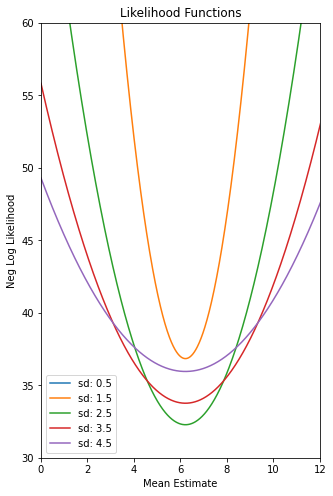
References
- Maximum Likelihood Estimation of Gaussian Parameters - Detailed derivation of MLE for Gaussian parameters
- Section 4.1 - Numerical computation - Deep Learning Book
- Bayes for beginners - probability and likelihood