Visualizing the regression function - the conditional mean
It is now instructive to go over an example to understand that even the plain-old mean squared error (MSE), the objective that is common in the regression setting, falls under the same umbrella - it’s the cross entropy between and a Gaussian model. Please follow the discussion associated with Section 5.5.1 of Ian Goodfellow’s Deep Learning book or section 20.2.4 of Russell & Norvig’s book and consider the following figure for assistance to visualize the relationship of and .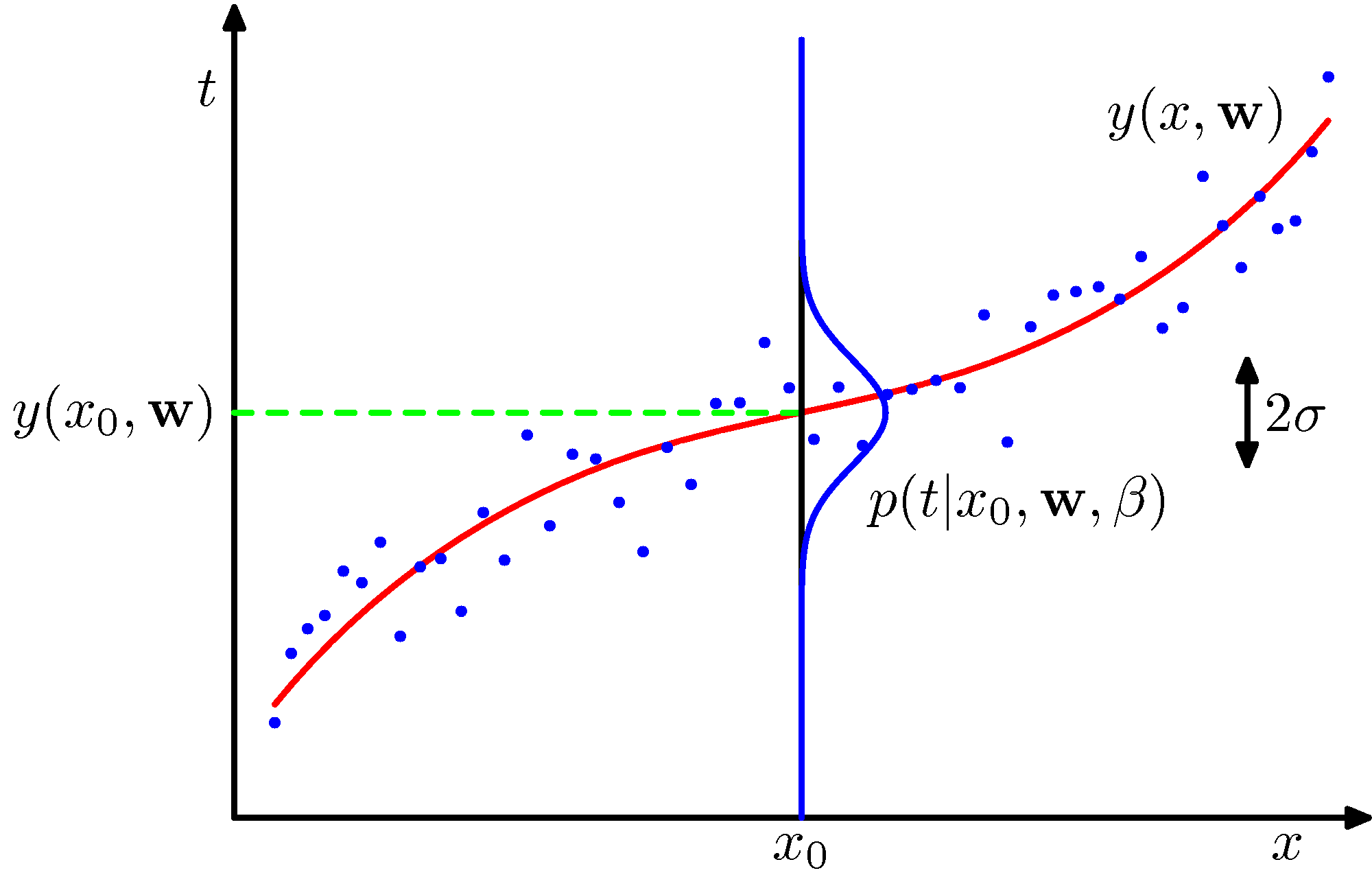
Key Insight: MSE as Cross-Entropy
When we assume the model distribution is Gaussian: The negative log-likelihood becomes: This is proportional to the mean squared error (MSE). Therefore, minimizing MSE is equivalent to maximum likelihood estimation under a Gaussian noise assumption.What the point estimate leaves out
Maximum likelihood returns a single , so it gives you one conditional-mean curve together with the fixed noise variance . Each of these is one source of predictive uncertainty:- The in the Gaussian is the aleatoric uncertainty. It is irreducible by construction: the model assumes the noise is constant, so it appears as the scaling and the additive const, never as something optimization can drive to zero.
- What a point estimate cannot show is how much the curve itself would shift if you refit on a different training sample. That spread is the epistemic uncertainty, and a single is silent about it.
References
- Marginal Maximum Likelihood - Introduction to MLE for marginal distributions
- MLE of Gaussian Parameters - Detailed derivation of MLE for Gaussian parameters
- Section 5.5.1 - Conditional Log-Likelihood - Deep Learning Book (Goodfellow, Bengio, Courville)
- Section 20.2.4 of Artificial Intelligence: A Modern Approach (Russell & Norvig)