Dataset Generation
We create a toy dataset by sampling from a sinusoidal function with added Gaussian noise: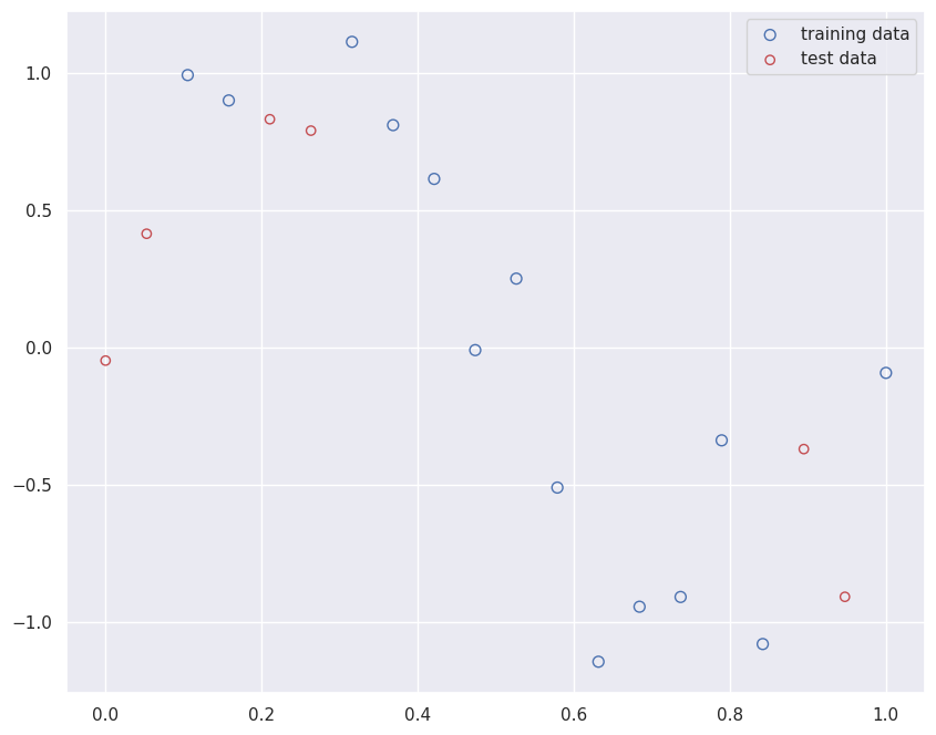
Polynomial Feature Transformation
We use polynomial features to enable fitting complex curves with linear regression: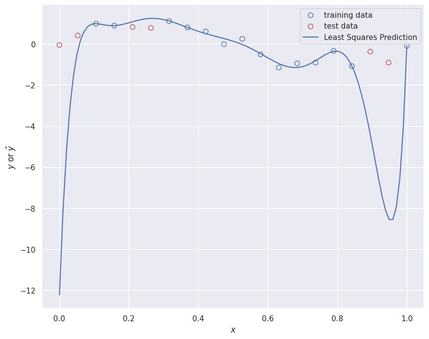
SGD Implementation with Regularization
The SGD loop implements mini-batch gradient descent with L2 regularization: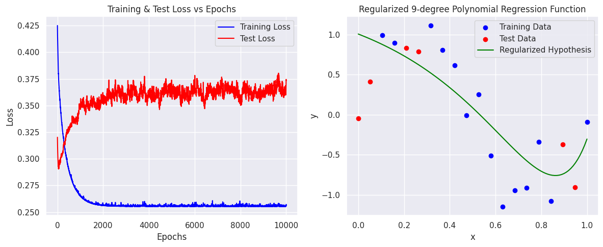
Hyperparameter Tuning with Optuna
We use Optuna to find the optimal regularization parameter :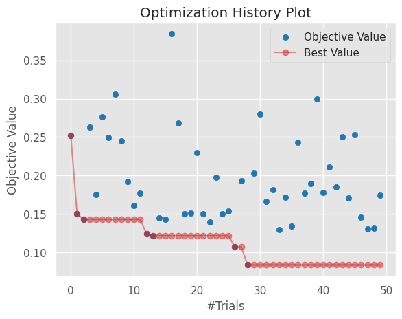
Key Takeaways
- Regularization prevents overfitting: High-degree polynomials (M=9) can memorize training data. L2 regularization constrains the weights to improve generalization.
- Learning rate matters: Too high causes divergence, too low causes slow convergence. A value of 0.01 works well for this problem.
- Batch size trade-offs: Larger batches give more stable gradients but slower updates per epoch. Full-batch gradient descent (batch_size = n_samples) is used for hyperparameter search stability.
- Automated tuning: Optuna efficiently searches the hyperparameter space using Bayesian optimization, finding good regularization values without manual grid search.
References
- Andrychowicz, M., Denil, M., Gomez, S., Hoffman, M., Pfau, D., et al. (2016). Learning to learn by gradient descent by gradient descent.
- Bottou, L., Curtis, F., Nocedal, J. (2016). Optimization Methods for Large-Scale Machine Learning.
- Keskar, N., Mudigere, D., Nocedal, J., Smelyanskiy, M., Tang, P. (2016). On Large-Batch Training for Deep Learning: Generalization Gap and Sharp Minima.
- Keskar, N., Mudigere, D., Nocedal, J., Smelyanskiy, M., Tang, P. (2016). On Large-Batch Training for Deep Learning: Generalization Gap and Sharp Minima.
- Martin-Maroto, F., Polavieja, G. (2018). Algebraic Machine Learning.