

 This section was written by Kimberly Milner (pull request #44), with help from an AI coding agent on the code. It reproduces the ideas of Chapter 6 of Foundations of Computer Vision by Antonio Torralba, Phillip Isola, and William T. Freeman. The book’s own figures are not reproduced here, because the book’s license covers only the work in full; links point to them instead.
This section answers a question pinholes cannot: how do you let in more light without sacrificing sharpness? The answer starts with Snell’s law. The first part derives the lensmaker’s formula, which turns Snell’s law plus a small-angle approximation into one equation,
relating object distance , image distance , and focal length .
Each figure is a runnable construction: change a refractive index, a radius of curvature, or an object distance, and the diagram redraws from the new physics. The book’s diagrams are regenerated directly. Where the book shows a photograph, either a synthetic version computed from the same physics stands in, or a link points to the book’s figure.
This section was written by Kimberly Milner (pull request #44), with help from an AI coding agent on the code. It reproduces the ideas of Chapter 6 of Foundations of Computer Vision by Antonio Torralba, Phillip Isola, and William T. Freeman. The book’s own figures are not reproduced here, because the book’s license covers only the work in full; links point to them instead.
This section answers a question pinholes cannot: how do you let in more light without sacrificing sharpness? The answer starts with Snell’s law. The first part derives the lensmaker’s formula, which turns Snell’s law plus a small-angle approximation into one equation,
relating object distance , image distance , and focal length .
Each figure is a runnable construction: change a refractive index, a radius of curvature, or an object distance, and the diagram redraws from the new physics. The book’s diagrams are regenerated directly. Where the book shows a photograph, either a synthetic version computed from the same physics stands in, or a link points to the book’s figure.
Introduction
A pinhole camera works: light from a scene passes through a small opening and forms an image on a sensor on the other side. But pinholes force a trade-off. Shrink the aperture and each scene point maps to a tight spot: the image is sharp, but so little light gets through that the image is dim. Open the aperture and more light arrives, but each scene point now spreads across many sensor pixels: the image is bright but blurry. There’s no single pinhole size that’s both sharp and bright. A lens breaks the trade-off. It gathers the wide cone of light a large aperture admits and refocuses it back to a single point on the sensor: bright like the wide pinhole, sharp like the narrow one. The rest of this section is the geometry of how a lens does that. Figure 6.1: Brightness/sharpness trade-offs in image formation. Three setups, same scene at the top, same sensor at the bottom. (a) Small pinhole: sharp image, very dim: little light reaches the sensor. (b) Large pinhole: bright image, very blurry: each scene point spreads to a wide disk at the sensor. (c) Lens: bright AND sharp: the lens collects a wide cone of light from each scene point and refocuses it to one sensor point. The book’s version is Figure 6.1; it demonstrates the same tradeoff with photographs in Figure 6.2.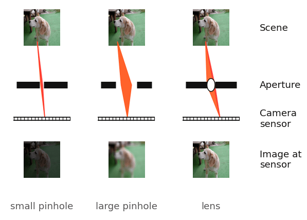
The lensmaker’s formula
A lens refracts light at each of its two surfaces. The lensmaker’s formula compresses that two-refraction process into one equation, relating object distance , image distance , and focal length . It follows from applying Snell’s law twice with the small-angle approximation : the paraxial regime where the algebra stays linear. For small angles in radians, , and Snell’s law at a glass-air interface (, ) becomes the linear . The book uses this paraxial form throughout the rest of the section. Figure 6.3(a): Snell’s law at a flat interface. A ray crosses from a medium with refractive index into a denser medium with and bends toward the normal. The angles are measured from the normal, and relates them. The book’s panel (b), a photograph of a straw refracting in a glass of water, is the same physics in the physical world; that photo is not reproduced here. (Book Figure 6.3.)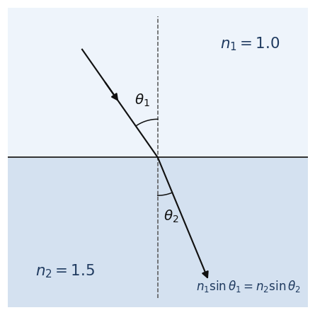
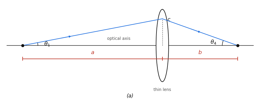
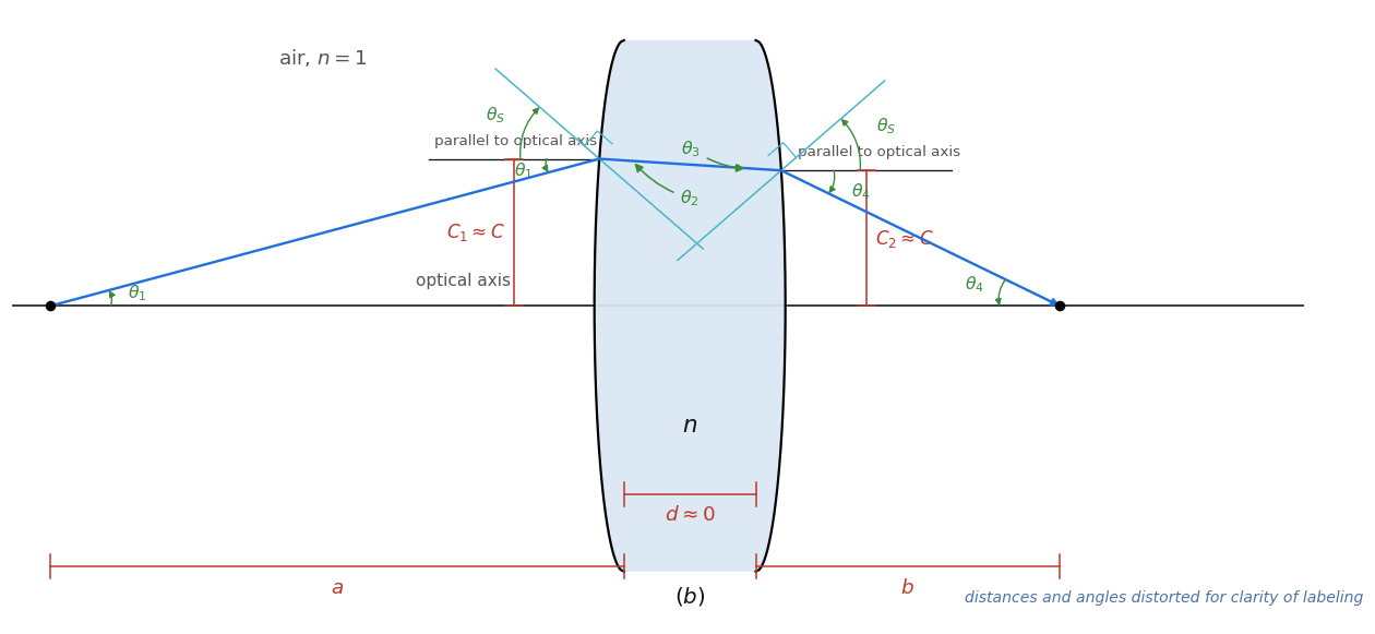
From flat interface to curved surface
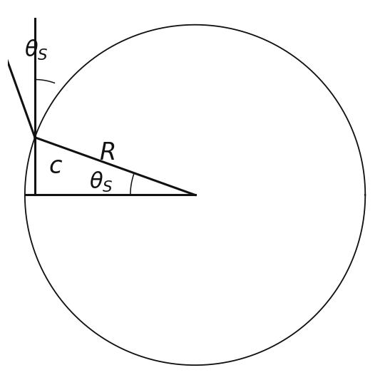
The angles in the lensmaker derivation are measured from each lens surface’s normal, but the lens’s surfaces aren’t flat: they’re spherical. Two things change with curvature. The normal at the point where a ray strikes the surface is no longer parallel to the optical axis, and the tilt of that normal depends on how far above the axis the ray hits. The next figure pins down that dependence: how the surface’s tilt angle relates to the radius of curvature and the hit height . Figure 6.5: Relation between and . A spherical surface of radius is drawn as a full circle centered on the optical axis. A ray meets the surface at height above the axis. The slanted radius from the center to that hit point makes an angle with the horizontal axis-radius: and the same angle reappears at the surface, between the vertical reference direction and the surface normal. In the small triangle formed by the slanted radius, the horizontal axis-radius, and the vertical leg of height , basic trigonometry gives . In the paraxial regime, this simplifies to which is exactly what thesurface_angle helper above returns, and what the lensmaker derivation in Figure 6.4(b) used at each surface. (Book Figure 6.5.)
Off-axis points
The derivation so far placed the object on the optical axis. Off-axis points need only a small extension: rotating the whole construction through a small angle adds to at each surface in Table 6.1, leaving the algebra unchanged. The lensmaker’s formula still holds, and the image lands at the conjugate distance on the far side, at height : inverted, below the axis. In the paraxial, thin-lens limit, this promotes the focusing property from points on an axis to whole planes: every point on the object plane at distance focuses to a corresponding point on the image plane at distance , both perpendicular to the optical axis. Figure 6.6: Off-axis points and the equivalent lens rotation. The off-axis object point sits at height above the optical axis, at distance from the lens; marks the on-axis reference. Two rays trace the image: a parallel ray refracts through the focal point at distance , and a ray through the lens center proceeds undeviated. They meet at the image point on the image plane at distance . The angle marks the small rotation that makes the off-axis case equivalent to the on-axis derivation. (Book Figure 6.6.)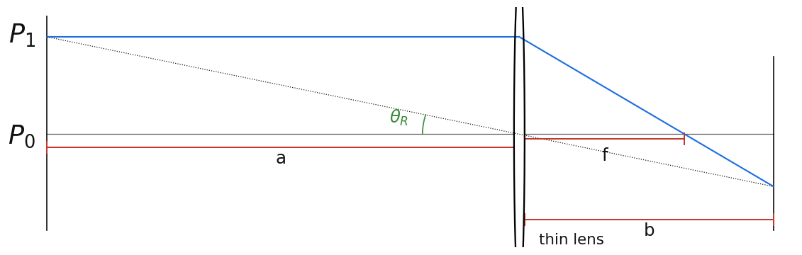
Imaging with lenses
With the lensmaker’s formula in hand, the rest of the chapter puts it to work: predicting where images form, how sharp they are, what changes with a concave lens, and how two lenses combine into a telescope. The starting observation is a small one, but it’s what lets the whole apparatus mimic a pinhole camera. At the very center of a thin lens, the front and back surfaces are parallel. A ray crossing that region refracts at the first surface, then refracts back through the same angle at the second surface: emerging parallel to the way it entered, displaced laterally by a small amount that depends on the lens’s thickness. In the thin-lens limit, the two surfaces collapse to a single plane: the displacement vanishes and the ray passes straight through. Every direction through the center is undeviated, which means the lens behaves, for those center rays, exactly like a pinhole: and a thin lens therefore images the world in perspective projection, just as a pinhole does. Figure 6.8: Rays through the center of a thin lens. (a) A physical lens of non-zero thickness: the ray refracts at both surfaces and exits parallel to the incoming direction, with a small lateral displacement. (b) The same ray under the thin-lens approximation: the two surfaces collapse to a single plane, the displacement vanishes, and the ray passes straight through. (c) Because every direction through the center is undeviated, a fan of rays through the lens center behaves identically to a fan of rays through a pinhole. (Book Figure 6.8.)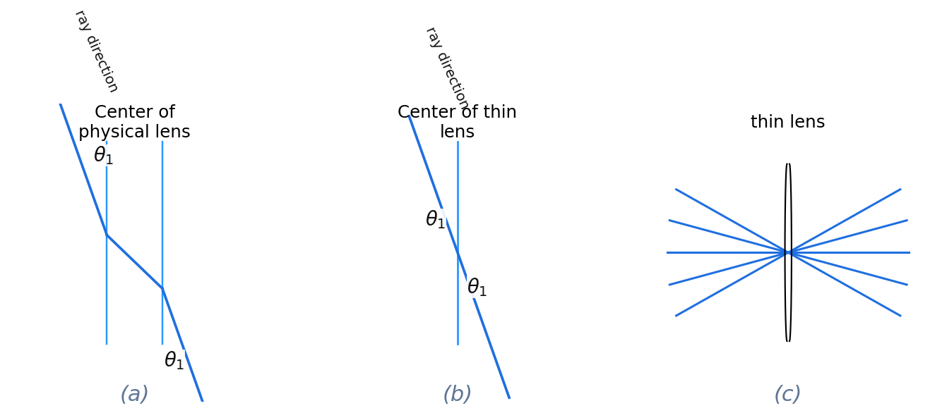
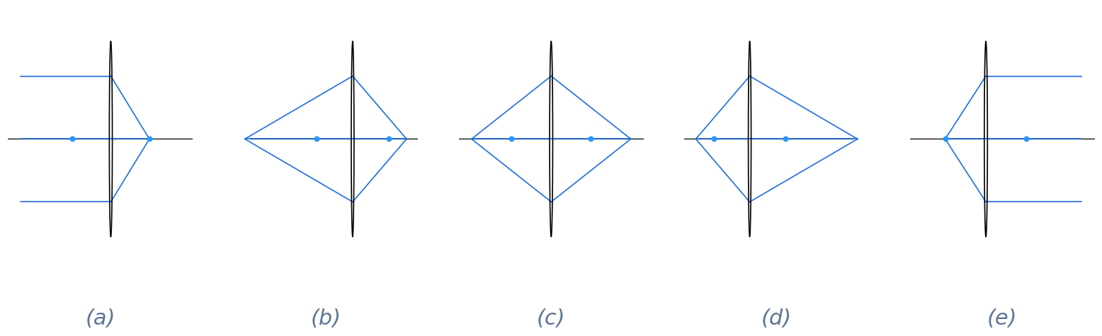
- Focusing: every ray from a point at distance reconverges at the conjugate distance , with .
- Parallel rays: the limit : parallel rays converge at the focal point, distance behind the lens.
- Center rays: any ray through the lens center proceeds in a straight line, as panel (c) above shows.
- Magnification: combining the first and third, a plane at distance images with scale : exactly as a pinhole at the lens center would project it.
Depth of field
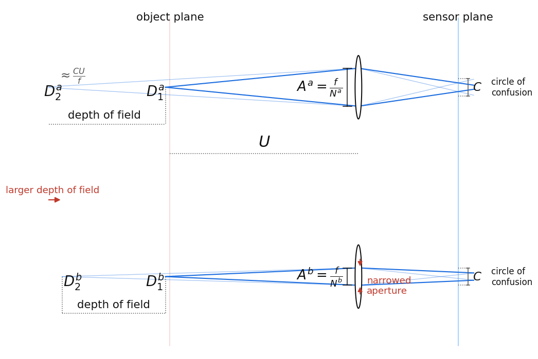
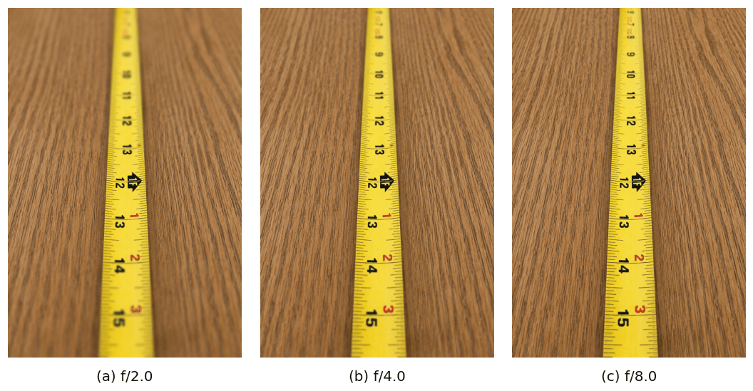
When the lens lives inside a camera, the sensor sits at a fixed distance behind it, so only one object distance is in sharp focus: the one whose conjugate is the sensor itself. That object distance defines an object plane (the focal plane in the book’s terminology) where everything images sharply. Objects in front of or behind that plane image past or before the sensor, hitting it as a small disk: a circle of confusion. A photograph still looks sharp as long as that circle is small enough that the eye can’t tell, and the range of object distances over which it stays acceptable is the depth of field. Figure 6.10: Circle of confusion and depth of field. Three object positions, one fixed sensor plane. The top row shows an object on the in-focus plane: every ray converges to a single point on the sensor for a sharp image. The middle row shows an object closer than the in-focus plane: its image forms past the sensor, hitting the sensor as a circle of confusion. The bottom row shows an object further than the in-focus plane: its image forms before the sensor, again hitting as a circle of confusion. The bracket on the left marks the depth of field. (Book Figure 6.10.)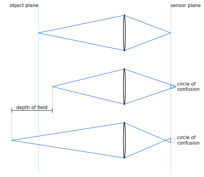
Concave lenses
The lens designed above was convex: both surfaces bowing outward, focal length positive. Reverse the curvature on both surfaces and you get a concave lens, with both surfaces bowing inward. In the lensmaker’s formula a concave surface contributes the same magnitude with the opposite sign, so comes out negative. The same paraxial geometry that focuses rays to a real point past a convex lens now bends them away from the axis at a concave lens: but the back-projection of those diverging rays still meets at a single point, on the source side of the lens. That point is the lens’s virtual focal point. Figure 6.13: Convex and concave thin-lens behavior. (a) A convex lens with focal length : parallel rays from the left converge to a real focal point at distance past the lens. (b) A concave lens with focal length : parallel rays diverge after the lens, but their back-projections (dotted) meet at a virtual focal point at distance on the source side. (c) Same concave lens with a tilted parallel bundle: the virtual focal point shifts off-axis (cyan), just as the focal point in a convex lens shifts to image off-axis sources: the lensmaker’s formula handles both cases with one sign change. (Book Figure 6.13.)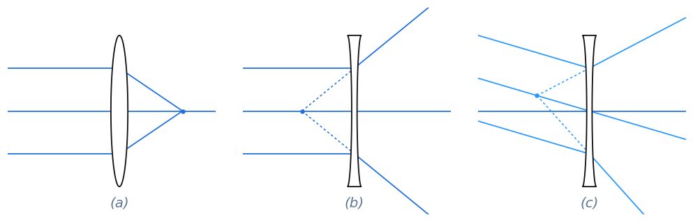
Lenses in a telescope
A convex lens and a concave lens together form a Galilean telescope, named after the one Galileo built in 1609. The construction is simple: place a convex lens (lens 1, focal length , long) with a concave lens (lens 2, focal length , shorter) such that they share a common focal point: lens 1 is distance to the left of that shared point, lens 2 is distance to the same side. The lenses sit apart. In that configuration, parallel rays entering lens 1 converge toward the shared focal point, and lens 2, intercepting them before they reach it, refracts them back into a parallel bundle. The output bundle is parallel like the input, but compressed into a smaller cross-section. What makes it a telescope is what happens when the input direction tilts. Figure 6.14: Galilean telescope geometry. (a) Parallel input, parallel output. Three parallel rays enter lens 1 from the left, converge toward the shared focal point, and are intercepted by lens 2 before reaching it: refracting back into a parallel bundle on the right. The output rays are parallel like the input, but closer together, compressed into the smaller exit aperture. (b) Tilted input, angular magnification. When the input bundle tilts at angle from the optical axis, the chief ray through lens 1’s center reaches the shared focal point at height above the axis (small-angle approximation, property 3 above). The same point is at distance from lens 2, which refracts the bundle into a parallel output at angle from the axis. The two similar triangles share the height but have different base lengths and , giving the magnification . (Book Figure 6.14.)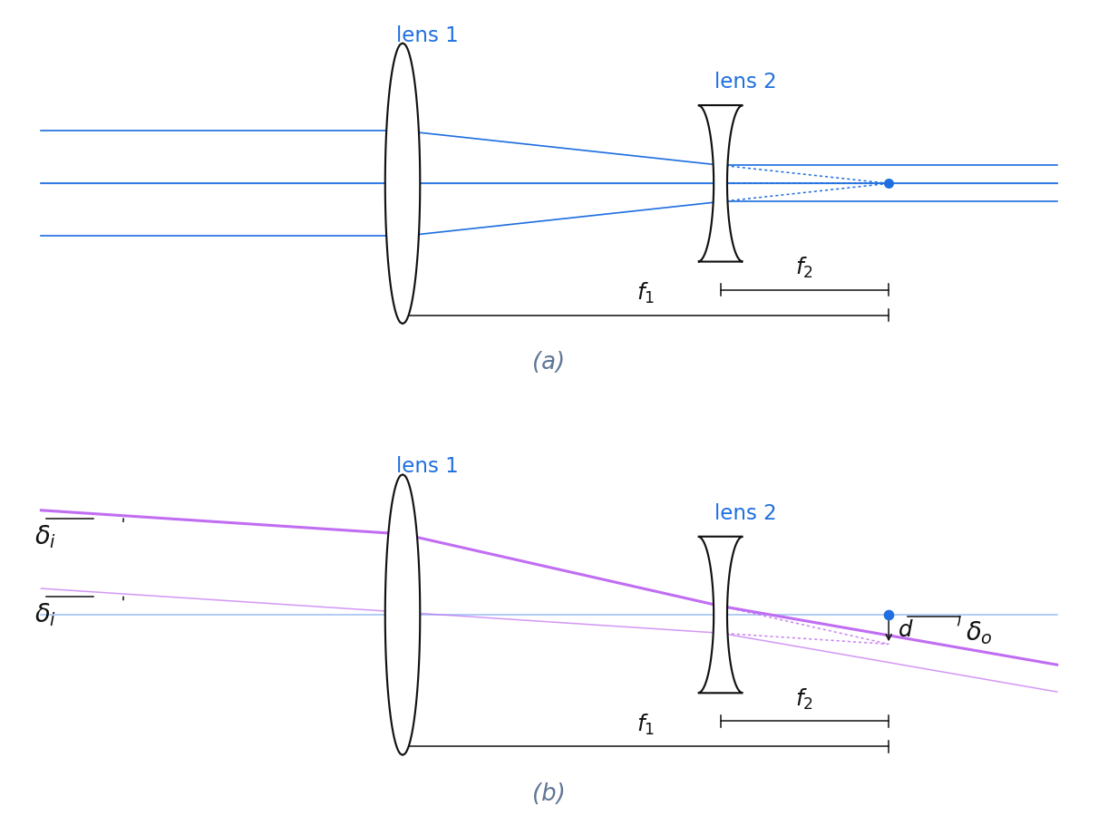
Found an error on this page? Report an issue.