Gradient descent
Optimization minimizes a function by adjusting . The derivative gives the slope: to first order , so moving a small step against the derivative decreases . For a vector of weights the gradient collects all partial derivatives, and gradient descent repeatedly steps downhill, where the learning rate scales the step. On a convex bowl the iterates march steadily to the unique minimum.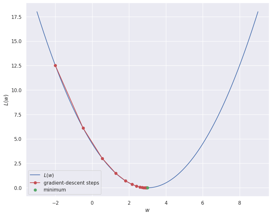
The learning rate
The learning rate sets the size of each step and is the most important knob. Too small and progress is glacial; too large and the steps overshoot the minimum and the iterates oscillate or diverge. For the quadratic above the update contracts the distance to the minimum by a factor per step, so anything with blows up.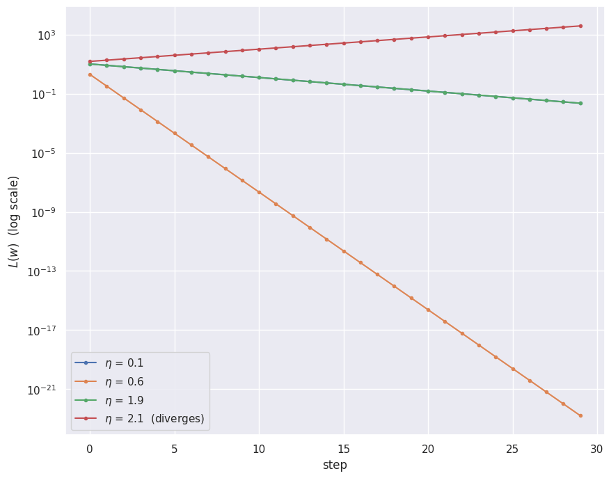
From full-batch to stochastic
In learning the loss is an average over the training set, and so is its gradient. For squared error with examples, Full-batch gradient descent sums over all examples for every single update. With millions of examples that is prohibitive. Instead you estimate the gradient on a random mini-batch of size ; the special case is stochastic gradient descent. The mini-batch gradient is an unbiased but noisy estimate of the full gradient, so each step is cheap and frequent, at the cost of a wandering trajectory. To see all three on one picture, fit a straight line to noisy data: the loss over the two parameters is a bowl whose contours you can draw.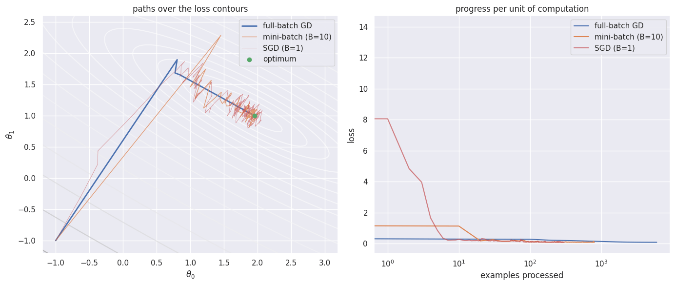
Gradient noise and learning-rate schedules
With a constant learning rate the stochastic gradient never vanishes, even at the optimum a single mini-batch still pulls in some direction. The iterate therefore settles into a noise ball around the minimum whose radius scales with , bouncing rather than converging. Shrinking the learning rate over time, for example , lets the ball contract so the iterate homes in. This is exactly the gap between the constant-rate and converged fits seen on the regression SGD example.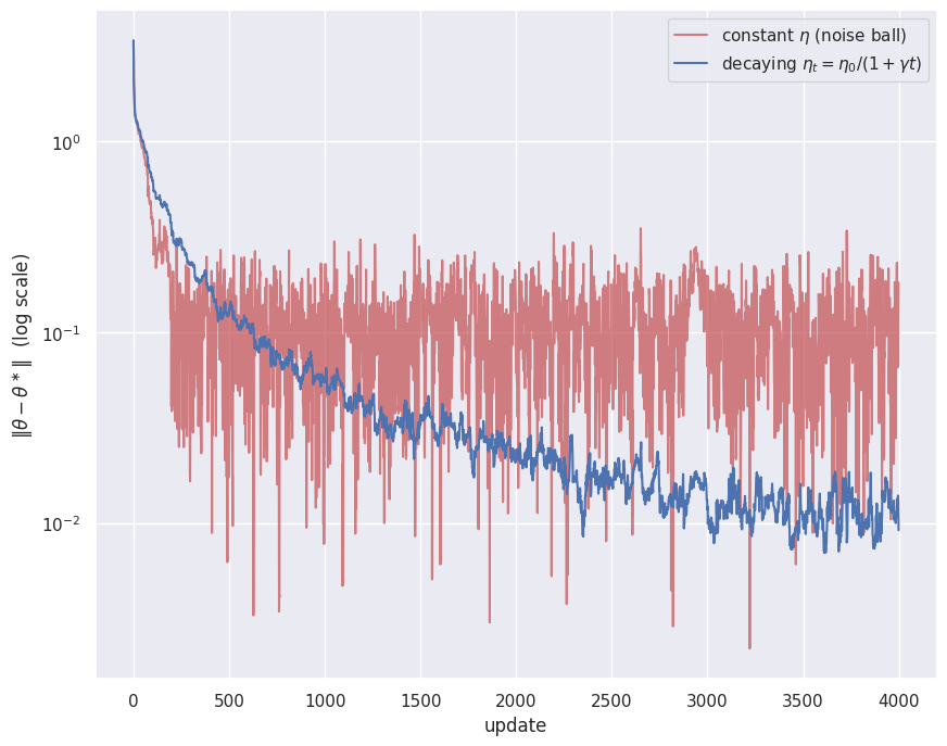
The same loop in PyTorch
Frameworks automate two things you did by hand: autograd computes from the forward computation, and an optimizer object applies the update rule. The mechanics are identical,loss.backward() fills in the gradient and optimizer.step() performs .
Takeaways
- Gradient descent steps against the gradient; the learning rate sets the step size, and too large a value diverges.
- The training loss is an average over data, so its gradient is too. Full-batch updates cost a complete pass, while mini-batch and stochastic updates trade gradient noise for cheap, frequent steps that make far more progress per unit of computation.
- A constant learning rate leaves stochastic gradient descent circling in a noise ball; a decaying schedule lets it converge.
- Autograd plus an optimizer object package this exact loop. The optimizer zoo section adds momentum and adaptive methods that handle the ill-conditioned, ravine-shaped landscapes where plain SGD struggles.
References
- Bottou, L., Curtis, F., Nocedal, J. (2016). Optimization Methods for Large-Scale Machine Learning.
- Goodfellow, I., Vinyals, O., Saxe, A. (2014). Qualitatively characterizing neural network optimization problems.