DDIM MoG Example - aegean.ai

Why DDIM

In the DDPM tutorial you trained a noise predictor

\epsilon_\theta(x_t, t)

and used the stochastic DDPM reverse chain to generate samples. Two practical pain points come up immediately:

It is slow. DDPM samples by stepping through every timestep $T \to T-1 \to \dots \to 1$ . With $T=500$ or $T=1000$ that is hundreds of network calls per sample.
It is non-deterministic. Even with a fixed initial noise $x_T$ , the reverse chain injects fresh noise at each step, so you cannot reproduce a specific sample or do clean latent interpolation.

DDIM (Song, Meng, Ermon, 2020) addresses both with a single trick: a non-Markovian forward process that has the same per-step marginals

q(x_t \mid x_0)

as DDPM. That means the same trained model

\epsilon_\theta

can be reused, but with a different sampler that:

Lets you skip timesteps (e.g. take 50 steps instead of 500, a 10× speedup).
Has a tunable noise level $\eta \in [0, 1]$ where $\eta = 1$ recovers DDPM and $\eta = 0$ is fully deterministic.

The deterministic case turns the diffusion model into an invertible map between Gaussian noise and data, which is what makes things like latent-space arithmetic and image editing possible.

Same target distribution as the DDPM tutorial

The 3-cluster MoG, seed 42, 300 points. We then train the same MLP noise predictor with the same DDPM objective.

import numpy as np
import torch
import torch.nn as nn
import torch.nn.functional as F
import matplotlib.pyplot as plt

torch.manual_seed(42)
np.random.seed(42)
device = torch.device("cuda" if torch.cuda.is_available() else "cpu")

n_samples = 300
cluster1 = np.random.multivariate_normal([0, 0], [[1, 0.5], [0.5, 1]], n_samples // 3)
cluster2 = np.random.multivariate_normal([6, 6], [[1.5, -0.7], [-0.7, 1.5]], n_samples // 3)
cluster3 = np.random.multivariate_normal([-4, 5], [[0.8, 0], [0, 2.0]], n_samples // 3)
data_np = np.vstack([cluster1, cluster2, cluster3]).astype(np.float32)
data = torch.from_numpy(data_np).to(device)

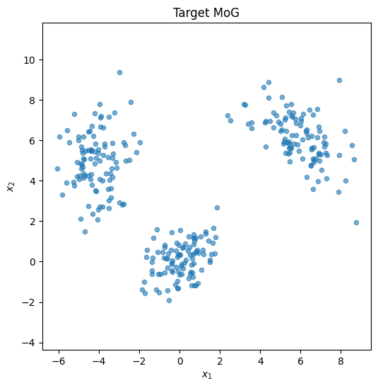
Forward (noising) process

Same fixed Markov noising chain as DDPM:

q(x_t \mid x_0) = \mathcal{N}\!\left(x_t;\sqrt{\bar\alpha_t}\,x_0,(1-\bar\alpha_t)I\right)

. We visualize a few specific timesteps so the noise schedule is concrete before training.

T = 500
betas = torch.linspace(1e-4, 0.02, T, device=device)
alphas = 1.0 - betas
alpha_bars = torch.cumprod(alphas, dim=0)

def q_sample(x0, t, eps=None):
    if eps is None:
        eps = torch.randn_like(x0)
    sqrt_ab = alpha_bars[t].sqrt().unsqueeze(-1)
    sqrt_omab = (1 - alpha_bars[t]).sqrt().unsqueeze(-1)
    return sqrt_ab * x0 + sqrt_omab * eps

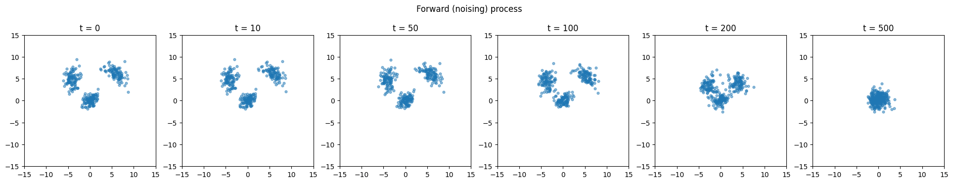
Train the noise predictor (same architecture and objective as DDPM)

DDIM and DDPM share the training step, only the sampler differs.

class SinusoidalTimeEmbedding(nn.Module):
    def __init__(self, dim):
        super().__init__()
        self.dim = dim

    def forward(self, t):
        half = self.dim // 2
        freqs = torch.exp(-np.log(10000) * torch.arange(half, device=t.device) / half)
        emb = t.float().unsqueeze(-1) * freqs
        return torch.cat([emb.sin(), emb.cos()], dim=-1)


class NoisePredictor(nn.Module):
    def __init__(self, time_dim=64, hidden=128):
        super().__init__()
        self.time_emb = nn.Sequential(
            SinusoidalTimeEmbedding(time_dim),
            nn.Linear(time_dim, time_dim), nn.SiLU(),
            nn.Linear(time_dim, time_dim),
        )
        self.net = nn.Sequential(
            nn.Linear(2 + time_dim, hidden), nn.SiLU(),
            nn.Linear(hidden, hidden), nn.SiLU(),
            nn.Linear(hidden, hidden), nn.SiLU(),
            nn.Linear(hidden, 2),
        )

    def forward(self, x, t):
        h = torch.cat([x, self.time_emb(t)], dim=-1)
        return self.net(h)


model = NoisePredictor().to(device)
optim = torch.optim.Adam(model.parameters(), lr=1e-3)
batch_size = 256
n_steps = 4000
losses = []

for step in range(n_steps):
    idx = torch.randint(0, data.shape[0], (batch_size,), device=device)
    x0 = data[idx]
    t = torch.randint(0, T, (batch_size,), device=device)
    eps = torch.randn_like(x0)
    xt = q_sample(x0, t, eps)
    eps_hat = model(xt, t)
    loss = F.mse_loss(eps_hat, eps)
    optim.zero_grad()
    loss.backward()
    optim.step()
    losses.append(loss.item())
    if (step + 1) % 1000 == 0:
        print(f"step {step + 1:>5d}  loss {float(np.mean(losses[-500:])):.4f}")

print("trained.")

step  1000  loss 0.5713

step  2000  loss 0.5401

step  3000  loss 0.5375

step  4000  loss 0.5341
trained.

The DDIM update rule

Given the trained

\epsilon_\theta

, define a strictly increasing sub-sequence

\tau = (\tau_1 < \tau_2 < \dots < \tau_S) \subseteq \{1, \dots, T\}

. The DDIM reverse step from

x_{\tau_i}

x_{\tau_{i-1}}

x_{\tau_{i-1}} = \sqrt{\bar\alpha_{\tau_{i-1}}} \,\hat x_0 \;+\; \sqrt{1 - \bar\alpha_{\tau_{i-1}} - \sigma_{\tau_i}^2}\; \epsilon_\theta(x_{\tau_i}, \tau_i) \;+\; \sigma_{\tau_i}\, z_{\tau_i}, \quad z_{\tau_i} \sim \mathcal{N}(0, I)

with the predicted clean sample

\hat x_0 = \frac{x_{\tau_i} - \sqrt{1-\bar\alpha_{\tau_i}}\, \epsilon_\theta(x_{\tau_i}, \tau_i)}{\sqrt{\bar\alpha_{\tau_i}}}

and the per-step noise scale

\sigma_{\tau_i} \;=\; \eta \, \sqrt{\frac{1-\bar\alpha_{\tau_{i-1}}}{1-\bar\alpha_{\tau_i}}} \, \sqrt{1 - \frac{\bar\alpha_{\tau_i}}{\bar\alpha_{\tau_{i-1}}}}

Two regimes:

$\eta = 1$ , full noise. The sampler becomes equivalent to DDPM (after accounting for sub-sequence corrections).
$\eta = 0$ , deterministic. The reverse step is a pure ODE-like update, $z_{\tau_i}$ disappears, and the same $x_T$ always produces the same $x_0$ .

Because the model was trained on the marginals

q(x_t \mid x_0)

(not the chain transitions), it does not care which sampler we use at inference time.

@torch.no_grad()
def ddim_sample(model, n=1000, n_steps=50, eta=0.0, x_T=None):
    """DDIM sampler.
    
    n_steps : length of the sub-sequence tau (uniform spacing across [0, T))
    eta     : 0.0 = deterministic, 1.0 = stochastic (≈ DDPM)
    x_T     : optional fixed initial noise (for reproducibility / interpolation)
    """
    if x_T is None:
        x = torch.randn(n, 2, device=device)
    else:
        x = x_T.clone()
        n = x.shape[0]

    taus = torch.linspace(0, T - 1, n_steps, device=device).long()
    taus = torch.unique(taus)

    for i in reversed(range(len(taus))):
        t_i = taus[i]
        ab_i = alpha_bars[t_i]
        ab_prev = alpha_bars[taus[i - 1]] if i > 0 else torch.tensor(1.0, device=device)

        eps = model(x, torch.full((x.shape[0],), t_i, device=device, dtype=torch.long))
        x0_hat = (x - (1 - ab_i).sqrt() * eps) / ab_i.sqrt()

        sigma = eta * ((1 - ab_prev) / (1 - ab_i)).sqrt() * (1 - ab_i / ab_prev).sqrt()
        dir_xt = (1 - ab_prev - sigma ** 2).clamp(min=0.0).sqrt() * eps
        noise = sigma * torch.randn_like(x) if i > 0 else torch.zeros_like(x)

        x = ab_prev.sqrt() * x0_hat + dir_xt + noise
    return x.cpu().numpy()

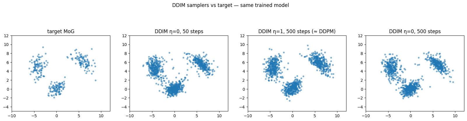
DDIM in 50 steps versus DDPM-equivalent in 500 steps

Three samplers, same model, 1000 generated points each:

DDIM η=0, 50 steps, fast, deterministic.
DDIM η=1, 500 steps, equivalent to DDPM, sanity check.
DDIM η=0, 500 steps, deterministic with the full timestep grid.

import time

def timed(fn, *args, **kw):
    if device.type == "cuda":
        torch.cuda.synchronize()
    start = time.time()
    out = fn(*args, **kw)
    if device.type == "cuda":
        torch.cuda.synchronize()
    return out, time.time() - start

samples_50_eta0,  t_50_eta0  = timed(ddim_sample, model, n=1000, n_steps=50,  eta=0.0)
samples_500_eta1, t_500_eta1 = timed(ddim_sample, model, n=1000, n_steps=500, eta=1.0)
samples_500_eta0, t_500_eta0 = timed(ddim_sample, model, n=1000, n_steps=500, eta=0.0)

print(f"DDIM eta=0, 50 steps  : {t_50_eta0*1000:6.1f} ms")
print(f"DDIM eta=1, 500 steps : {t_500_eta1*1000:6.1f} ms  (≈ DDPM)")
print(f"DDIM eta=0, 500 steps : {t_500_eta0*1000:6.1f} ms")

DDIM eta=0, 50 steps  :   87.3 ms
DDIM eta=1, 500 steps :  335.1 ms  (≈ DDPM)
DDIM eta=0, 500 steps :  343.1 ms

Determinism: same noise, same sample

With

\eta = 0

the sampler is a deterministic function of the initial noise

x_T

. Run it twice with the same

x_T

and you get bit-identical outputs, regardless of how many steps you take.

x_T = torch.randn(500, 2, device=device)
out_a = ddim_sample(model, n_steps=50, eta=0.0, x_T=x_T)
out_b = ddim_sample(model, n_steps=50, eta=0.0, x_T=x_T)
max_abs_diff = float(np.max(np.abs(out_a - out_b)))
print(f"max |x_a - x_b| = {max_abs_diff:.3e} (should be 0 with eta=0)")

x_T2 = torch.randn(500, 2, device=device)
out_c = ddim_sample(model, n_steps=50, eta=0.0, x_T=x_T2)

max |x_a - x_b| = 0.000e+00 (should be 0 with eta=0)

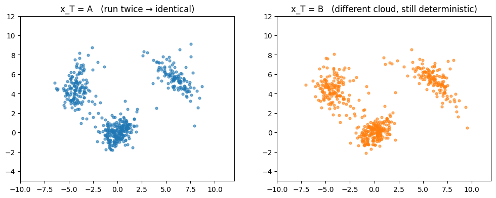
Latent interpolation: slerp on $x_T$

Because

\eta = 0

DDIM is a deterministic invertible map, you can pick two endpoints in noise space and walk a path between them; each intermediate noise decodes to a coherent point in data space. The right path on the unit sphere is spherical linear interpolation (slerp), which preserves the Gaussian magnitude.

def slerp(z0, z1, t):
    """Spherical linear interpolation in 2D Gaussian noise space."""
    z0_n = z0 / z0.norm()
    z1_n = z1 / z1.norm()
    omega = torch.acos((z0_n * z1_n).sum().clamp(-1.0, 1.0))
    so = torch.sin(omega)
    return (torch.sin((1 - t) * omega) / so) * z0 + (torch.sin(t * omega) / so) * z1

torch.manual_seed(0)
z_a = torch.randn(2, device=device)
z_b = torch.randn(2, device=device)
n_path = 50
ts = torch.linspace(0, 1, n_path)
path = torch.stack([slerp(z_a, z_b, float(t)) for t in ts], dim=0).to(device)
decoded = ddim_sample(model, n_steps=50, eta=0.0, x_T=path)

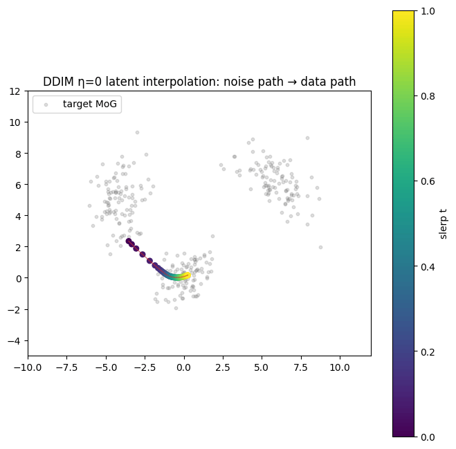
Connections to other concepts

Sampler decoupling. Training trains; sampling samples. DDIM proves you can swap samplers freely as long as marginals are preserved. Modern stacks ship many samplers (DDIM, DPM-Solver, Euler, Heun, …) on top of the same DDPM-trained network.
Step count is a knob, not a constant. Image-generation pipelines routinely use 20-50 DDIM steps in production where DDPM would take 1000.
Deterministic = invertible. $\eta = 0$ DDIM gives you a noise-to-data map you can run forwards and backwards, enabling editing and interpolation.
Bridge to flows and ODEs. Deterministic DDIM is the discretization of a probability-flow ODE. That connection underlies most of the recent diffusion-model speedup work (consistency models, rectified flow, …).
Score-based unification. The Score MoG Tutorial makes that ODE bridge concrete: train $s_\theta(x, \sigma)$ on the same MoG, then sample via annealed Langevin or the reverse-time SDE. Deterministic DDIM is the probability-flow ODE limit of that score-SDE.

References

Song, Meng, Ermon. Denoising Diffusion Implicit Models. ICLR 2021. arxiv.org/abs/2010.02502
Ho, Jain, Abbeel. Denoising Diffusion Probabilistic Models. NeurIPS 2020. arxiv.org/abs/2006.11239
Song et al. Score-Based Generative Modeling through Stochastic Differential Equations. ICLR 2021. arxiv.org/abs/2011.13456

Edit this page on GitHub or file an issue.

​Why DDIM

​Same target distribution as the DDPM tutorial

​Forward (noising) process

​Train the noise predictor (same architecture and objective as DDPM)

​The DDIM update rule

​DDIM in 50 steps versus DDPM-equivalent in 500 steps

​Determinism: same noise, same sample

​Latent interpolation: slerp on xTx_TxT​

​Connections to other concepts

​References

Why DDIM

Same target distribution as the DDPM tutorial

Forward (noising) process

Train the noise predictor (same architecture and objective as DDPM)

The DDIM update rule

DDIM in 50 steps versus DDPM-equivalent in 500 steps

Determinism: same noise, same sample

Latent interpolation: slerp on $x_T$

Connections to other concepts

References