Score MoG Example - aegean.ai

The target distribution

The same 2D Mixture of Gaussians used by the DDPM, DDIM, and Brownian motion tutorials: three anisotropic Gaussians, seed 42, 300 points total. To DDPM you trained a noise predictor

\epsilon_\theta

. Here you train a score predictor

s_\theta(x, \sigma)

that approximates

\nabla_x \log p_\sigma(x)

, the gradient of the log-density of the data after Gaussian smoothing at scale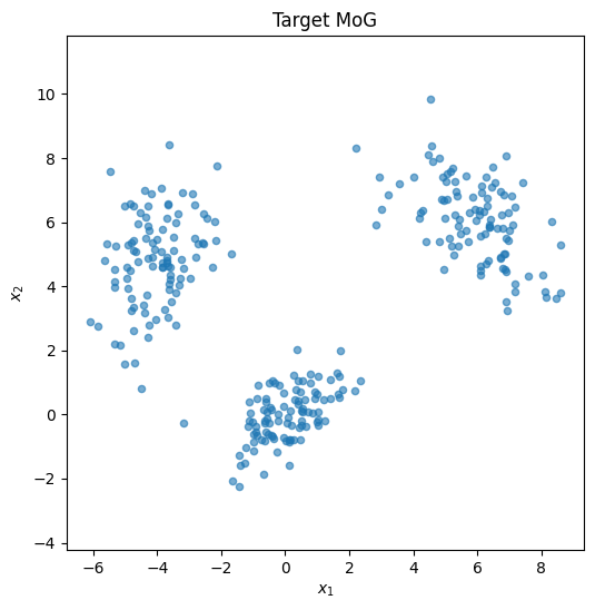

\sigma

import numpy as np
import torch
import torch.nn as nn
import torch.nn.functional as F
import matplotlib.pyplot as plt

torch.manual_seed(42)
np.random.seed(42)
device = torch.device("cuda" if torch.cuda.is_available() else "cpu")

n_samples = 300
components = [
    {"mean": np.array([0.0, 0.0]),  "cov": np.array([[1.0, 0.5], [0.5, 1.0]])},
    {"mean": np.array([6.0, 6.0]),  "cov": np.array([[1.5, -0.7], [-0.7, 1.5]])},
    {"mean": np.array([-4.0, 5.0]), "cov": np.array([[0.8, 0.0], [0.0, 2.0]])},
]
weights = np.array([1.0, 1.0, 1.0]) / 3.0

rng = np.random.default_rng(42)
data_np = np.vstack([
    rng.multivariate_normal(c["mean"], c["cov"], n_samples // 3) for c in components
]).astype(np.float32)
data = torch.from_numpy(data_np).to(device)

Denoising score matching

We perturb data with Gaussian noise at scale

\sigma

\tilde x = x + \sigma\, \epsilon, \qquad \epsilon \sim \mathcal{N}(0, I)

The score of the smoothed density satisfies

\nabla_{\tilde x} \log p_\sigma(\tilde x \mid x) = -\frac{\tilde x - x}{\sigma^2} = -\frac{\epsilon}{\sigma}

so the denoising score-matching objective

L = \mathbb{E}_{x, \sigma, \epsilon}\!\left[\,\sigma^2 \big\| s_\theta(\tilde x, \sigma) + \epsilon / \sigma \big\|^2\,\right]

trains

s_\theta(\tilde x, \sigma)

to estimate

\nabla \log p_\sigma(\tilde x)

across a range of noise scales. The

\sigma^2

weighting makes the loss balanced across scales, Song & Ermon 2019. We use a logarithmic noise schedule

\sigma \in [\sigma_{\min}, \sigma_{\max}]

with

\sigma_{\min} = 0.05

\sigma_{\max} = 5.0

SIGMA_MIN, SIGMA_MAX = 0.05, 5.0

def sample_sigma(n):
    """Log-uniform sample of sigma for DSM training."""
    u = torch.rand(n, device=device)
    return SIGMA_MIN * (SIGMA_MAX / SIGMA_MIN) ** u


class ScoreNet(nn.Module):
    """Small MLP s_theta(x, sigma). Conditions on log(sigma) via sinusoidal embedding."""
    def __init__(self, sigma_dim=64, hidden=128):
        super().__init__()
        self.sigma_dim = sigma_dim
        self.net = nn.Sequential(
            nn.Linear(2 + sigma_dim, hidden), nn.SiLU(),
            nn.Linear(hidden, hidden), nn.SiLU(),
            nn.Linear(hidden, hidden), nn.SiLU(),
            nn.Linear(hidden, 2),
        )

    def sigma_emb(self, sigma):
        half = self.sigma_dim // 2
        freqs = torch.exp(-np.log(10000) * torch.arange(half, device=sigma.device) / half)
        emb = torch.log(sigma).unsqueeze(-1) * freqs
        return torch.cat([emb.sin(), emb.cos()], dim=-1)

    def forward(self, x, sigma):
        return self.net(torch.cat([x, self.sigma_emb(sigma)], dim=-1))


model = ScoreNet().to(device)
optim = torch.optim.Adam(model.parameters(), lr=2e-3)

Training

Standard DSM loop: sample a batch, sample a per-example

\sigma

, perturb, predict the score, minimize the noise-conditional loss.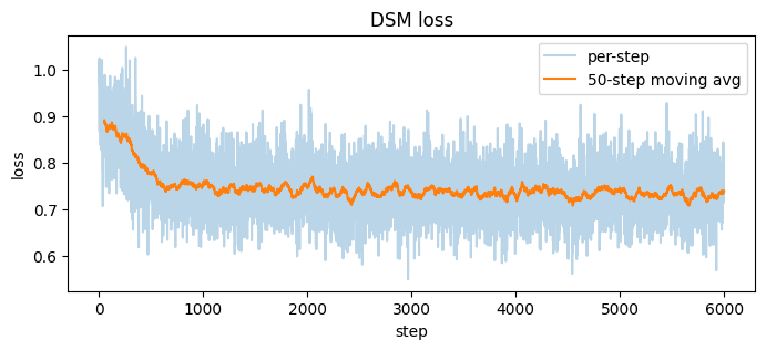

batch_size = 256
n_steps = 6000
losses = []

for step in range(n_steps):
    idx = torch.randint(0, data.shape[0], (batch_size,), device=device)
    x0 = data[idx]
    sigma = sample_sigma(batch_size)
    eps = torch.randn_like(x0)
    xt = x0 + sigma.unsqueeze(-1) * eps
    target = -eps / sigma.unsqueeze(-1)
    pred = model(xt, sigma)
    loss = ((sigma.unsqueeze(-1) * (pred - target)) ** 2).mean()
    optim.zero_grad(); loss.backward(); optim.step()
    losses.append(loss.item())
    if (step + 1) % 1500 == 0:
        print(f"step {step + 1:>5d}  loss {float(np.mean(losses[-500:])):.4f}")

print("trained.")

step  1500  loss 0.7443

step  3000  loss 0.7404

step  4500  loss 0.7398

step  6000  loss 0.7311
trained.

The learned score field

Evaluate

s_\theta

on a grid at low noise (

\sigma = 0.3

), at this scale the score points toward the data manifold, so the field should converge into the three MoG modes.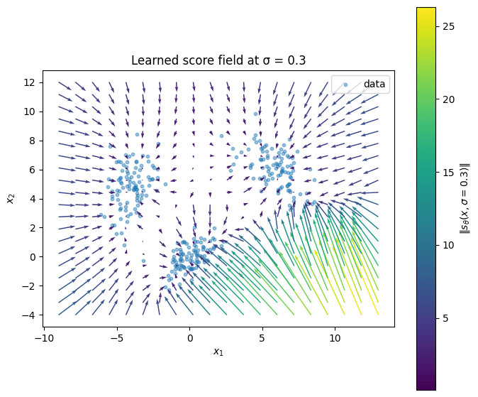

@torch.no_grad()
def score_grid(sigma_val=0.3, lo=(-9, -4), hi=(13, 12), n=20):
    xs = torch.linspace(lo[0], hi[0], n, device=device)
    ys = torch.linspace(lo[1], hi[1], n, device=device)
    X, Y = torch.meshgrid(xs, ys, indexing="xy")
    pts = torch.stack([X.flatten(), Y.flatten()], dim=-1)
    sigma = torch.full((pts.shape[0],), sigma_val, device=device)
    s = model(pts, sigma)
    return X.cpu().numpy(), Y.cpu().numpy(), s[:, 0].view(n, n).cpu().numpy(), s[:, 1].view(n, n).cpu().numpy()

X, Y, U, V = score_grid()

Above: the analytical score field $\nabla \log p(x)$ for this MoG, manimgl-rendered. Compare with the matplotlib quiver of the learned $s_\theta$ , both should pull mass toward the three component centers.

Annealed Langevin sampling

Generate samples by running Langevin dynamics at decreasing noise levels:

x_{k+1} = x_k + \alpha_k\, s_\theta(x_k, \sigma_k) + \sqrt{2\alpha_k}\, z_k, \quad z_k \sim \mathcal{N}(0, I)

with step size

\alpha_k = \epsilon \cdot \sigma_k^2 / \sigma_{\min}^2

, Song & Ermon’s recipe. Larger

\sigma

steps cover broad regions of space; smaller

\sigma

steps refine onto the data manifold.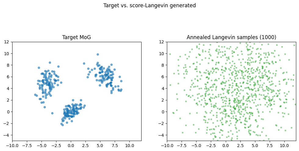

@torch.no_grad()
def annealed_langevin(n=1000, n_sigmas=10, n_inner=8, eps=2e-5):
    sigmas = torch.from_numpy(
        np.geomspace(SIGMA_MAX, SIGMA_MIN, n_sigmas).astype(np.float32)
    ).to(device)
    x = torch.randn(n, 2, device=device) * SIGMA_MAX + torch.tensor([2.0, 4.0], device=device)
    for sigma in sigmas:
        alpha = eps * (sigma ** 2) / (SIGMA_MIN ** 2)
        sigma_b = sigma.expand(n)
        for _ in range(n_inner):
            s = model(x, sigma_b)
            x = x + alpha * s + torch.sqrt(2 * alpha) * torch.randn_like(x)
    return x.cpu().numpy()

samples_langevin = annealed_langevin(n=1000)

Above: 80 particles released uniformly, then annealed-Langevin-stepped through a geometric noise schedule from $\sigma = 2.5$ down to $\sigma = 0.15$ . The cloud condenses into the three MoG components.

Reverse-time SDE

The variance-exploding (VE) SDE has forward

dx_t = \sqrt{\frac{d[\sigma_t^2]}{dt}}\, dW_t

and reverse-time form

dx_t = -\frac{d[\sigma_t^2]}{dt}\, s_\theta(x_t, \sigma_t)\, dt + \sqrt{\frac{d[\sigma_t^2]}{dt}}\, d\bar W_t

Discretize with Euler-Maruyama from

t = 1

down to

t = 0

. This is the same chain as DDIM at

\eta = 1

in the score-SDE framework.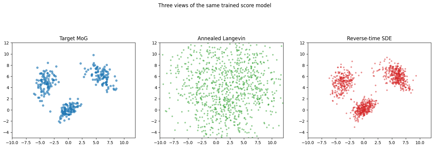

@torch.no_grad()
def reverse_sde(n=1000, n_steps=400):
    """Euler-Maruyama on the reverse VE-SDE with learned score."""
    ts = torch.linspace(1.0, 0.0, n_steps + 1, device=device)
    sigmas = SIGMA_MIN * (SIGMA_MAX / SIGMA_MIN) ** ts
    x = torch.randn(n, 2, device=device) * sigmas[0] + torch.tensor([2.0, 4.0], device=device)
    for i in range(n_steps):
        sigma = sigmas[i]
        sigma_next = sigmas[i + 1]
        # d[sigma^2] over this Δt is sigma^2 - sigma_next^2 (positive going forward in time)
        d_sigma2 = (sigma ** 2 - sigma_next ** 2).clamp(min=0)
        sigma_b = sigma.expand(n)
        s = model(x, sigma_b)
        x = x + d_sigma2 * s + torch.sqrt(d_sigma2) * torch.randn_like(x)
    return x.cpu().numpy()

samples_sde = reverse_sde(n=1000)

Above: 60 particles seeded broadly, evolving under the reverse-time SDE driven by the analytical MoG score. Trails show each particle’s path as it condenses into one of the three modes.

Connections to other concepts

Score-matching is the unifying view. DDPM’s noise predictor $\epsilon_\theta$ is, up to the scaling $-1/\sigma$ , a score predictor; DDIM’s deterministic sampler is the probability-flow ODE limit of the same score-SDE. The framework above subsumes both.
Sampler decoupling. Once you have $s_\theta$ , you can swap samplers: annealed Langevin, reverse SDE, probability-flow ODE, predictor-corrector. The trained network is unchanged.
The information-theoretic angle. $s_\theta(x, t)$ is the local geometry of $\log p_t(x)$ , the same quantity that, integrated through Fisher-information identities, gives mutual information bounds. See AURA-672 for the score → Fisher → MI thread.

References

Song, Ermon. Generative Modeling by Estimating Gradients of the Data Distribution. NeurIPS 2019. arxiv.org/abs/1907.05600
Song, Sohl-Dickstein, Kingma, Kumar, Ermon, Poole. Score-Based Generative Modeling through Stochastic Differential Equations. ICLR 2021. arxiv.org/abs/2011.13456
Vincent. A Connection Between Score Matching and Denoising Autoencoders. Neural Computation 2011.

Edit this page on GitHub or file an issue.

​The target distribution

​Denoising score matching

​Training

​The learned score field

​Annealed Langevin sampling

​Reverse-time SDE

​Connections to other concepts

​References

The target distribution

Denoising score matching

Training

The learned score field

Annealed Langevin sampling

Reverse-time SDE

Connections to other concepts

References