Open In Colab Plain gradient descent, the subject of the previous section, struggles on two landscape features that are very common. In a ravine, where the loss curves far more sharply in one direction than another, it zigzags across the steep walls while creeping along the shallow floor. Near a saddle point, where the gradient nearly vanishes, it stalls. This section builds the standard fixes from scratch, momentum, Nesterov, RMSProp, and Adam, compares their trajectories on both landscapes, and then shows the same optimizers through torch.optim. Throughout, θ\boldsymbol{\theta} is the parameter vector and g=θL\mathbf{g} = \nabla_{\boldsymbol{\theta}} L is the gradient.

A ravine

Take an anisotropic quadratic that is steep in one coordinate and shallow in the other, L(θ)=12(θ02+κθ12),θL=(θ0,  κθ1).L(\boldsymbol{\theta}) = \tfrac{1}{2}\big(\theta_0^2 + \kappa\,\theta_1^2\big), \qquad \nabla_{\boldsymbol{\theta}} L = (\theta_0,\; \kappa\,\theta_1). The Hessian has eigenvalues 11 and κ\kappa, so the condition number is κ\kappa. Gradient descent is stable only while η<2/κ\eta < 2/\kappa, set by the steep direction, but then the shallow direction contracts by just (1η)(1 - \eta) per step. With κ\kappa large the steep coordinate oscillates while the shallow one barely moves: the familiar zigzag down a narrow valley.
KAPPA = 100.0
def L(theta):
    return 0.5 * (theta[0]**2 + KAPPA * theta[1]**2)
def grad(theta):
    return np.array([theta[0], KAPPA * theta[1]])

start = np.array([-9.0, -1.0])     # common starting point; minimum is at the origin
print(f"condition number kappa = {KAPPA:.0f}")
condition number kappa = 100

Momentum

Momentum accumulates a running velocity v\mathbf{v} that averages successive gradients. Oscillating components (the steep direction) cancel, while the consistent component (the shallow floor) builds up, so the iterate accelerates along the valley instead of bouncing across it: vt=μvt1+gt,θt=θt1ηvt,\mathbf{v}_t = \mu\,\mathbf{v}_{t-1} + \mathbf{g}_t, \qquad \boldsymbol{\theta}_t = \boldsymbol{\theta}_{t-1} - \eta\,\mathbf{v}_t, with momentum coefficient μ[0,1)\mu \in [0,1). Nesterov momentum evaluates the gradient at a look-ahead point θ+μv\boldsymbol{\theta} + \mu\mathbf{v}, which corrects overshoot and usually converges a little faster.

Adaptive methods: RMSProp and Adam

A different fix rescales each coordinate by its own recent gradient magnitude, so steep directions take smaller steps and shallow directions larger ones automatically. RMSProp keeps an exponential average of squared gradients s\mathbf{s} and divides by its root, st=ρst1+(1ρ)gt2,θt=θt1ηst+ϵgt.\mathbf{s}_t = \rho\,\mathbf{s}_{t-1} + (1-\rho)\,\mathbf{g}_t^2, \qquad \boldsymbol{\theta}_t = \boldsymbol{\theta}_{t-1} - \frac{\eta}{\sqrt{\mathbf{s}_t} + \epsilon}\,\mathbf{g}_t. Adam combines this with momentum, tracking averages of both the gradient (m\mathbf{m}) and its square (v\mathbf{v}), each bias-corrected, mt=β1mt1+(1β1)gt,vt=β2vt1+(1β2)gt2,θt=θt1ηm^tv^t+ϵ.\mathbf{m}_t = \beta_1\mathbf{m}_{t-1} + (1-\beta_1)\mathbf{g}_t, \quad \mathbf{v}_t = \beta_2\mathbf{v}_{t-1} + (1-\beta_2)\mathbf{g}_t^2, \quad \boldsymbol{\theta}_t = \boldsymbol{\theta}_{t-1} - \eta\,\frac{\hat{\mathbf{m}}_t}{\sqrt{\hat{\mathbf{v}}_t} + \epsilon}. Each optimizer below is a small step function that reads and updates its own state; a shared runner iterates it and records the path.
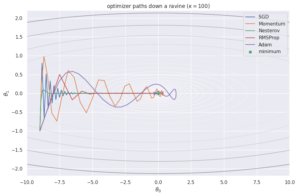
def run(step, grad, theta0, n=120):
    theta, state, path = np.array(theta0, float), {}, [np.array(theta0, float)]
    for t in range(1, n + 1):
        theta = step(theta, grad, state, t)
        path.append(theta.copy())
    return np.array(path)

def sgd(lr):
    def step(th, grad, s, t):
        return th - lr * grad(th)
    return step

def momentum(lr, mu=0.9):
    def step(th, grad, s, t):
        s["v"] = mu * s.get("v", 0.0) + grad(th)
        return th - lr * s["v"]
    return step

def nesterov(lr, mu=0.9):
    def step(th, grad, s, t):
        v = s.get("v", np.zeros_like(th))
        v = mu * v - lr * grad(th + mu * v)
        s["v"] = v
        return th + v
    return step

def rmsprop(lr, rho=0.99, eps=1e-8):
    def step(th, grad, s, t):
        g = grad(th)
        s["s"] = rho * s.get("s", 0.0) + (1 - rho) * g**2
        return th - lr * g / (np.sqrt(s["s"]) + eps)
    return step

def adam(lr, b1=0.9, b2=0.999, eps=1e-8):
    def step(th, grad, s, t):
        g = grad(th)
        s["m"] = b1 * s.get("m", 0.0) + (1 - b1) * g
        s["v"] = b2 * s.get("v", 0.0) + (1 - b2) * g**2
        mhat, vhat = s["m"] / (1 - b1**t), s["v"] / (1 - b2**t)
        return th - lr * mhat / (np.sqrt(vhat) + eps)
    return step
paths = {
    "SGD":      run(sgd(0.018),      grad, start),
    "Momentum": run(momentum(0.012, 0.85), grad, start),
    "Nesterov": run(nesterov(0.008, 0.85), grad, start),
    "RMSProp":  run(rmsprop(0.15),   grad, start),
    "Adam":     run(adam(0.5),       grad, start),
}
for name, p in paths.items():
    print(f"{name:9s} final L = {L(p[-1]):.3g}")
SGD       final L = 0.518
Momentum  final L = 2e-07
Nesterov  final L = 2.71e-07
RMSProp   final L = 6.49e-11
Adam      final L = 9.05e-07
Output from cell 5

Saddle points

In high dimensions most critical points where the gradient vanishes are not minima but saddles, low along some directions and high along others. A clean two-dimensional model is L(θ)=12(θ02θ12),θL=(θ0,  θ1),L(\boldsymbol{\theta}) = \tfrac{1}{2}\big(\theta_0^2 - \theta_1^2\big), \qquad \nabla_{\boldsymbol{\theta}} L = (\theta_0,\; -\theta_1), with a saddle at the origin. Starting almost on the ridge (θ10\theta_1 \approx 0) the gradient in the escape direction is tiny, so plain gradient descent and momentum dawdle near the origin, while the per-coordinate scaling in RMSProp and Adam amplifies the weak direction and breaks away sooner.
def L_saddle(theta):
    return 0.5 * (theta[0]**2 - theta[1]**2)
def grad_saddle(theta):
    return np.array([theta[0], -theta[1]])

start_s = np.array([-1.8, 1e-2])     # almost on the ridge
paths_s = {
    "SGD":      run(sgd(0.08),      grad_saddle, start_s, n=35),
    "Momentum": run(momentum(0.04), grad_saddle, start_s, n=35),
    "RMSProp":  run(rmsprop(0.03),  grad_saddle, start_s, n=35),
    "Adam":     run(adam(0.05),     grad_saddle, start_s, n=35),
}
for name, p in paths_s.items():
    print(f"{name:9s} |theta_1| after 35 steps = {abs(p[-1, 1]):.3f}")
SGD       |theta_1| after 35 steps = 0.148
Momentum  |theta_1| after 35 steps = 1.752
RMSProp   |theta_1| after 35 steps = 4.711
Adam      |theta_1| after 35 steps = 1.958
Output from cell 7

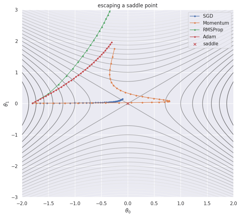
The same optimizers in PyTorch

torch.optim ships these as one-line choices. Vanilla SGD takes a momentum argument, and Adam is its own class. Optimizing the ravine through autograd reproduces what you built by hand.
import torch

def torch_descend(make_opt, n=120):
    theta = torch.tensor([-9.0, -1.0], requires_grad=True)
    opt = make_opt([theta])
    loss = None
    for _ in range(n):
        opt.zero_grad()
        loss = 0.5 * (theta[0]**2 + KAPPA * theta[1]**2)
        loss.backward()
        opt.step()
    return theta.detach().numpy(), loss.item()

for name, make_opt in {
    "SGD":          lambda p: torch.optim.SGD(p, lr=0.018),
    "SGD+momentum": lambda p: torch.optim.SGD(p, lr=0.012, momentum=0.85),
    "Adam":         lambda p: torch.optim.Adam(p, lr=0.5),
}.items():
    theta, loss = torch_descend(make_opt)
    print(f"{name:13s} final L = {loss:.3g}   theta = {np.round(theta, 3)}")
SGD           final L = 0.537   theta = [-1.018 -0.   ]
SGD+momentum  final L = 4.64e-07   theta = [ 0.001 -0.   ]
Adam          final L = 5.66e-05   theta = [-0.001 -0.   ]

Takeaways

  • Plain gradient descent is limited by the steepest direction, so on an ill-conditioned ravine it zigzags and the shallow direction crawls.
  • Momentum averages gradients into a velocity that cancels the oscillation and accelerates along the valley; Nesterov sharpens this with a look-ahead gradient.
  • Adaptive methods (RMSProp, Adam) rescale each coordinate by its own gradient history, which both fixes the conditioning and helps escape saddle points where one direction is nearly flat.
  • Adam is momentum plus per-coordinate scaling with bias correction, the common default; well-tuned SGD with momentum often matches or beats it on large problems.
  • torch.optim provides all of these; the update rules are exactly the ones implemented here by hand.
Key references: (Kingma & Ba, 2014; Ruder2016-overview; Goodfellow et al., 2014)

References

  • Goodfellow, I., Vinyals, O., Saxe, A. (2014). Qualitatively characterizing neural network optimization problems.
  • Kingma, D., Ba, J. (2014). Adam: A Method for Stochastic Optimization.