Predicting the load of the electrical grid

In this example, we’ll fit a degree-9 polynomial to a small sample of real MISO grid load using stochastic gradient descent (SGD). The loss is the same regularized ridge objective solved in closed form on the linear regression page; the difference is that SGD works toward the solution one update at a time. Instead of guessing the regularization strength

\lambda

, we’ll use an outer Optuna search to find the value

\lambda^\ast

with the lowest held-out error.

The dataset

We’ll treat one day of grid load as a regression problem. The input

x

is the normalized time of day, and the target

y

is the total load across the MISO system. After fetching the data from the gridstatus.io API, we standardize it to zero mean and unit variance. We then keep just ten readings for training. That tiny sample is intentional: it gives a degree-9 polynomial plenty of room to overfit, just as it did in the closed-form example. The rest of the day’s readings are held out so we can evaluate each value of

\lambda

MISO, the Midcontinent Independent System Operator, manages the wholesale electricity market and balances electricity supply and demand across 15 US states and Manitoba. The curve below shows one real day from the gridstatus.io MISO load dataset, fetched through the gridstatus API.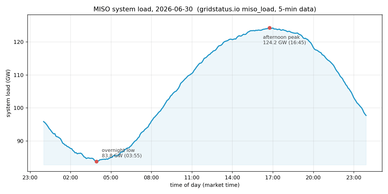

MISO system load versus time for 2026-06-30 from gridstatus.io, rising from an overnight low near 84 GW to an afternoon peak near 124 GW

Real MISO system load on 2026-06-30, using five-minute readings from the gridstatus.io miso_load dataset.Forecast errors have real consequences here. Grid operators schedule generation ahead of time, but supply and demand must stay balanced from moment to moment. If a forecast is too low, operators may need emergency power purchases and, in severe cases, load shedding. If it is too high, they may commit expensive generators that were not needed. A model that follows noise instead of the underlying demand pattern can therefore make the grid harder and more expensive to operate.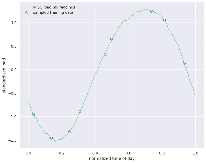

# Fetch one real day of MISO system load from the gridstatus.io API.
# GRIDSTATUS_API_KEY is read from the environment (.env); it is never hardcoded.
import logging
logging.getLogger("gridstatusio").setLevel(logging.WARNING)
load_dotenv()
client = GridStatusClient(os.environ["GRIDSTATUS_API_KEY"])
df = client.get_dataset(
    dataset="miso_load",
    start="2026-06-30",
    end="2026-07-01",
    timezone="market",
    verbose=False,
)

t = pd.to_datetime(df["interval_start_local"])
secs = (t - t.min()).dt.total_seconds().to_numpy()
x_all = secs / secs.max()                       # normalized time of day in [0, 1]
load_gw = df["load"].to_numpy() / 1000.0        # system load in GW

# Standardize the target so the learning rate and lambda stay on a familiar (unit-variance) scale.
y_mean, y_std = load_gw.mean(), load_gw.std()
y_all = (load_gw - y_mean) / y_std

# A deliberately small training set (like the original ten-point toy set); the rest of the
# day is held out to score lambda.
rng = np.random.default_rng(1)
train_idx = np.sort(rng.choice(len(x_all), size=10, replace=False))
mask = np.ones(len(x_all), bool); mask[train_idx] = False
x_train, y_train = x_all[train_idx], y_all[train_idx]
x_val,   y_val   = x_all[mask],     y_all[mask]

Standardized polynomial features

Our model is a degree-9 polynomial,

g(x;\boldsymbol{\theta}) = \bar{y} + \sum_{k=1}^{9}\theta_k\,\phi_k(x).

The raw terms

x, x^2, \dots, x^9

have very different scales on

[0,1]

. As a result, one gradient step can affect some coefficients far more than others, and the penalty

\lambda\lVert\boldsymbol{\theta}\rVert^2

does not act evenly across them. We avoid that problem by standardizing every feature to zero mean and unit variance. A single learning rate and a single value of

\lambda

then make sense for all nine coefficients. This also matches the feature scaling used on the closed-form page, so the two results can be compared directly. We handle the intercept separately by centering the targets at

\bar{y}

M = 9
P_train = np.vander(x_train, M + 1, increasing=True)[:, 1:]   # columns x^1 .. x^9
mu, sd = P_train.mean(0), P_train.std(0) + 1e-12

def featurize(xq):
    P = np.vander(np.ravel(xq), M + 1, increasing=True)[:, 1:]
    return (P - mu) / sd

Phi_train = featurize(x_train)
Phi_val = featurize(x_val)              # the rest of the day, held out to score lambda
y_bar = y_train.mean()                  # intercept; SGD fits the centered residual

The regularized objective and the SGD update

SGD minimizes the same ridge objective that the closed-form solution minimizes: the sum of squared residuals plus an

\ell_2

penalty.

J(\boldsymbol{\theta}) = \sum_{i=1}^{n}\big(\boldsymbol{\phi}_i^{\top}\boldsymbol{\theta} - \tilde{y}_i\big)^2 + \lambda\lVert\boldsymbol{\theta}\rVert^2, \qquad \tilde{y}_i = y_i - \bar{y}.

The minimum satisfies the normal equations

(\boldsymbol{\Phi}^{\top}\boldsymbol{\Phi} + \lambda\mathbf{I})\boldsymbol{\theta} = \boldsymbol{\Phi}^{\top}\tilde{\mathbf{y}}

. Because both methods use this convention,

\lambda

has the same meaning here as it does in the closed-form solution. At each step, SGD draws a mini-batch

\mathcal{B}

containing

B

examples. Multiplying the batch sum by

n/B

gives us an unbiased estimate of the full gradient:

\boldsymbol{\theta} \leftarrow \boldsymbol{\theta} - \eta\Big(\tfrac{2n}{B}\,\boldsymbol{\Phi}_{\mathcal{B}}^{\top}(\boldsymbol{\Phi}_{\mathcal{B}}\boldsymbol{\theta} - \tilde{\mathbf{y}}_{\mathcal{B}}) + 2\lambda\boldsymbol{\theta}\Big).

def sgd_fit(lam, lr=0.004, epochs=20000, batch_size=5, seed=0):
    g = np.random.default_rng(seed)
    yc = y_train - y_bar                # centered target
    n = len(y_train)
    theta = np.zeros(M)
    train_hist, val_hist = [], []
    for _ in range(epochs):
        order = g.permutation(n)
        for s in range(0, n, batch_size):
            b = order[s:s + batch_size]
            err = Phi_train[b] @ theta - yc[b]
            grad = (2 * n / len(b)) * (Phi_train[b].T @ err) + 2 * lam * theta
            theta -= lr * grad
        res = Phi_train @ theta - yc
        train_hist.append(np.sum(res**2) + lam * np.sum(theta**2))
        val_hist.append(np.mean((Phi_val @ theta + y_bar - y_val) ** 2))
    return theta, np.array(train_hist), np.array(val_hist)

Finding a good value for $\lambda$

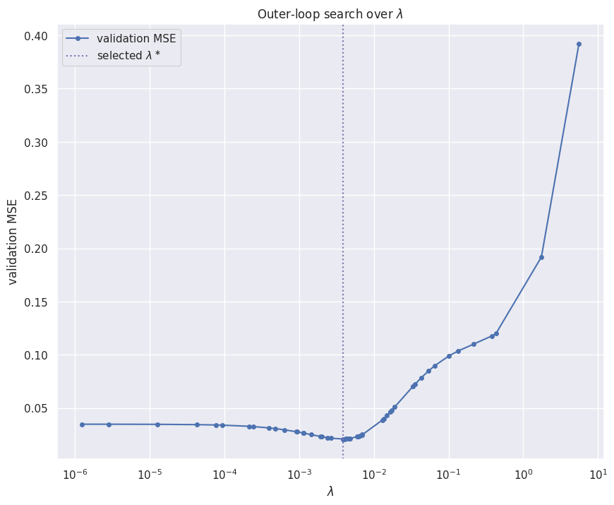
The training loss cannot tell us how much regularization to use. It will always favor

\lambda \to 0

, since weaker shrinkage lets the polynomial fit the ten training points more closely. To choose

\lambda

based on how well the model generalizes, we use two loops:

In the inner loop, SGD trains the degree-9 model for one fixed value of $\lambda$ and returns its error on the held-out readings.
In the outer loop, Optuna proposes values of $\lambda$ across a wide logarithmic range. It uses the validation error from each inner run to decide what to try next.

The value with the lowest held-out error becomes

\lambda^\ast

. It is selected from this grid-load dataset rather than copied from the earlier example.

import warnings
warnings.filterwarnings("ignore")
import optuna
optuna.logging.set_verbosity(optuna.logging.WARNING)

def objective(trial):
    # outer loop proposes lambda over a wide range; inner loop is a full SGD fit
    lam = trial.suggest_float("lambda", 1e-6, 1e1, log=True)
    _, _, val_hist = sgd_fit(lam)
    return float(np.mean(val_hist[-200:]))      # validation MSE of the converged model

study = optuna.create_study(direction="minimize", sampler=optuna.samplers.TPESampler(seed=0))
study.optimize(objective, n_trials=50)

lambda_star = study.best_params["lambda"]
print(f"selected lambda*     : {lambda_star:.2e}")
print(f"validation MSE at it : {study.best_value:.4f}")

selected lambda*     : 3.89e-03
validation MSE at it : 0.0209

Comparing the two solutions

Once the search has found

\lambda^\ast

, we train the degree-9 model one more time and compare its SGD weights with the closed-form ridge solution at the same value of

\lambda

. The two fits should be nearly identical. They minimize the same objective; they simply take different routes to get there.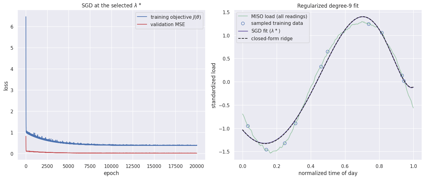

theta_sgd, train_hist, val_hist = sgd_fit(lambda_star)

# closed-form ridge at the selected lambda, for comparison
theta_cf = np.linalg.solve(
    Phi_train.T @ Phi_train + lambda_star * np.eye(M), Phi_train.T @ (y_train - y_bar))

xq = np.linspace(0, 1, 200)
gap = np.max(np.abs(featurize(xq) @ theta_sgd - featurize(xq) @ theta_cf))
print(f"validation MSE at lambda*           : {val_hist[-1]:.4f}")
print(f"max |SGD - closed-form| over [0, 1] : {gap:.3f}")

validation MSE at lambda*           : 0.0207
max |SGD - closed-form| over [0, 1] : 0.007

What to take away

Choosing $\lambda$ is a model-selection problem. Optuna tries candidate values in the outer loop, while SGD trains and evaluates a model in the inner loop. Training loss alone is not enough because it always favors less shrinkage.
The regularization term contributes $2\lambda\boldsymbol{\theta}$ to the gradient. This shrinks the weights at every update and helps keep the degree-9 polynomial from overfitting.
When SGD and the closed-form method use the same standardized features and the same $\lambda^\ast$ , they reach the same regularized solution.
On this grid-load sample, the search settles near $4\times10^{-3}$ . That is close in scale to the $3.04\times10^{-3}$ found for the unit-variance sinusoid on the closed-form page, even though the value was tuned independently.

Key references: (Keskar et al., 2016; Bottou et al., 2016; Andrychowicz et al., 2016)

References

Andrychowicz, M., Denil, M., Gomez, S., Hoffman, M., Pfau, D., et al. (2016). Learning to learn by gradient descent by gradient descent.
Bottou, L., Curtis, F., Nocedal, J. (2016). Optimization Methods for Large-Scale Machine Learning.
Keskar, N., Mudigere, D., Nocedal, J., Smelyanskiy, M., Tang, P. (2016). On Large-Batch Training for Deep Learning: Generalization Gap and Sharp Minima.

Edit this page on GitHub or file an issue.

Foundations

Learning & Regression

Optimization

Maximum Likelihood

Classification

Dimensionality Reduction

Predicting the load of the electrical grid

The dataset

Standardized polynomial features

The regularized objective and the SGD update

Finding a good value for $\lambda$

Comparing the two solutions

What to take away

References

​The dataset

​Standardized polynomial features

​The regularized objective and the SGD update

​Finding a good value for λ\lambdaλ

​Comparing the two solutions

​What to take away

​References

The dataset

Standardized polynomial features

The regularized objective and the SGD update

Finding a good value for $\lambda$

Comparing the two solutions

What to take away

References