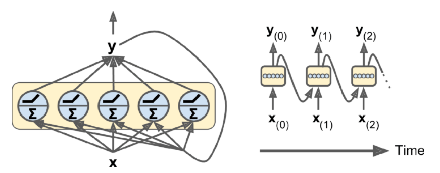
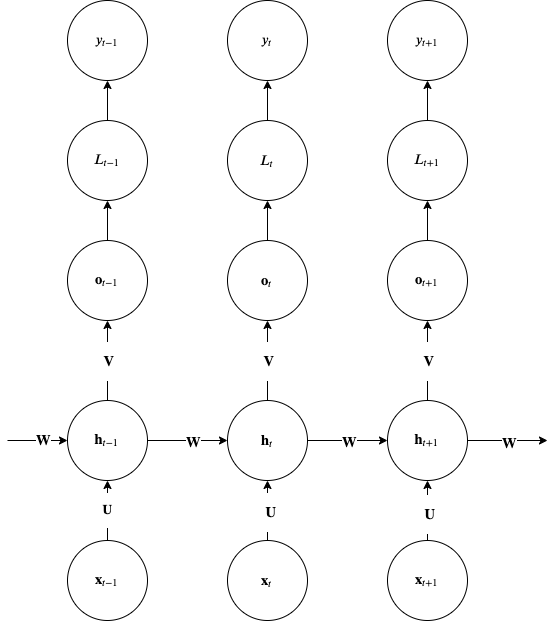
The simplest RNN has a single layer of neurons that receive the input x.Simple RNN layer with nneurons RNN neurons that map the input to the hidden state at each time step.A more practical simple RNN adds recurrences between the hidden units and an output at every step.Simple RNN with recurrences between hidden units. This architecture can compute any computable function, so it is as powerful as a Universal Turing Machine.Notice how the input xt−1 affects the label yt through the hidden state. Notice also that the outputs y are conditionally independent of each other given the inputs x.
To use this diagram for backpropagation, swap the roles of its nodes and edges. In a computational graph the tensors sit on the edges and the RNN functions (gates) sit in the nodes.
Dimensioning simple RNNs
In the table below, m is the number of examples in the mini-batch.
Variable
Dimensions
ht
nneurons×1 or m×nneurons
xt
ninput×1 or m×ninput
U
nneurons×ninput
W
nneurons×nneurons
b
nneurons×1
V
noutput×nneurons
o
noutput×1
c
noutput×1
You can stack several such layers on top of each other. Each layer keeps its own hidden state.
Forward propagation
This network maps an input sequence to an output sequence of the same length. Its forward pass is:athtoty^t=Wht−1+Uxt+b=tanh(at)=Vht+c=softmax(ot)The time series forecasting section implements the first two lines as a small PyTorch module and checks it against nn.RNN.The loss over a sequence of length τ is the KL divergence between the empirical distribution of the data and the model distribution. Up to a constant that does not depend on θ, it is the negative log-likelihood:L=DKL[p^data(y∣x)∥pmodel(y∣x;θ)]=−Ey∣x∼p^datalogpmodel(y∣x;θ)=−t∑logpmodel(yt∣x1,…,xt;θ)where L is shorthand for L(y^1,…,y^τ,y1,…,yτ).RNNs can model very general distributions logpmodel(x,y;θ). The simple RNN above models the conditional distribution logpmodel(y∣x;θ). Because of the conditional independence assumption, that distribution factorizes into ∑tlogpmodel(yt∣x1,…,xt;θ).
You can remove this simplifying assumption by connecting yt−1 to ht through another matrix, for example R. The network can then model an arbitrary distribution logpmodel(y∣x;θ). As in other deep network architectures, the connectivity directly affects the representational capacity of the hypothesis set.
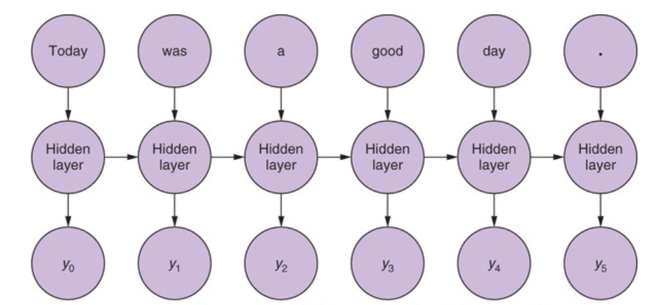
In many problems only the label yτ at the end of the sequence matters. Suppose you classify speech or video from inside a car cabin to detect the psychological state of the driver. The same architecture covers this case: you keep only oτ, Lτ and yτ and ignore the outputs at earlier steps.An example makes the forward equations concrete.Example sentence as input to the RNNThe figure shows a short document (a sentence) broken into tokens. Here a token is a word, and the sentence has τ=6 tokens. Suppose you need one label for the whole document. At t=1 the network receives the first token x1. Starting from the hidden state h0=0, it computes h1 with the forward equations and ignores the output o1. It repeats this unrolling for each new input x2,x3,… until it reaches the end-of-sentence token x6. Only at that step does it compute the output y6 and the loss−logpmodel(y6∣x1,…,x6;θ)where θ={W,U,V,b,c}.
Backpropagation through time (BPTT)
Training uses backpropagation on the unrolled network.Understanding RNN memory through the BPTT procedureBackpropagation in an RNN looks like backpropagation in other networks, because the unrolled architecture resembles a feed-forward one. There is one important difference, which the computational graph above shows for recurrences t−1 and t. The computation of ht uses the value ht−1 from the previous recurrence. When you apply the chain rule in the backward pass, every node that involves such a recurrent variable receives a non-local gradient from a later step (t in the figure). In the networks you have seen so far, each gate only used gradients local to it.This is why a simple RNN is said to have memory. Look at the backward pass in recurrence t−1, at the junction between tanh and Vht−1. The gradient ∇ht−1Lt arrives there from the backpropagation of the Wht−1 node in recurrence t. Because the node is a junction, this gradient is added to the gradient that flows down from the output of recurrence t−1:∇ht−1Lt−1←∇ht−1Lt−1+∇ht−1LtSection 10.2.2 of Goodfellow, Bengio and Courville gives the exact equations. The intuition behind the computational graph is enough to follow the rest of this chapter.In practice BPTT is truncated. Without truncation, a single gradient update would need a full forward pass and a full backward pass over the training sequence, which for a language model is very long. If the truncation length is too short, the bias it introduces can stop SGD from converging. The truncation length is usually chosen by a heuristic, larger than the expected memory of the system, or by cross-validation.PyTorch runs BPTT for you: calling backward() on a loss computed from an unrolled nn.RNN sends the gradient back through every step. The time series forecasting section trains simple and deep RNNs this way to predict the next values of a series.
Vanishing or exploding gradients
The figure below is a conceptual picture of a recurrence over time. It is called an infinite impulse response (IIR) filter, for reasons that become clear shortly.Infinite impulse response (IIR) filter with weight wLet D denote a unit delay, a memory location that stores a value for one step. The recurrence of this system isht=wht−1+xtwhere w is a scalar weight. Feed an impulse xt=δt into the system with w=−0.9:h0h1h2h3=−0.9h−1+δ0=1=−0.9h0+δ1=−0.9=−0.9h1+δ2=0.81=−0.9h2+δ3=−0.729With w=−0.9, the impulse response ht follows a decaying exponential envelope. With ∣w∣>1 it would follow a growing exponential envelope. If the recurrence continues, the response vanishes or explodes long after the impulse entered at t=0. In this simple filter, the weight alone decides which of the two happens.
The RNN hidden-state recurrence behaves the same way in the backward pass, which runs from t=τ back to t=1. When τ is large, the gradient can vanish or explode. The scalar w of the IIR filter becomes the matrix W, and the signal h becomes the gradient ∇htLt. Pascanu, Mikolov and Bengio analyze this in detail.The derivative of the tanh non-linearity, shown below, lies between 0 and 1. It shrinks the gradients and slows down training.Derivative of the tanh non-linearityThe repeated multiplication by W has a similar effect. If you ignore the non-linearity, the hidden state is ht=Wht−1, so after τ stepshτ=Wτh0The same power of W appears in the expression for ∇htLt (see section 10.2.2). If the magnitudes of the eigenvalues of W are below 1, the gradients vanish. If they are above 1, the gradients explode. The long short-term memory (LSTM) architecture in the next section addresses this problem.
Key references: (Graves et al., n.d.; Jaderberg et al., 2016; Parisotto et al., 2016)
References
Graves, A., Wayne, G., Danihelka, I. (n.d.). Neural Turing Machines. Link
Jaderberg, M., Czarnecki, W., Osindero, S., Vinyals, O., Graves, A., et al. (2016). Decoupled Neural Interfaces using Synthetic Gradients. arXiv [cs.LG]. Link
Parisotto, E., Mohamed, A., Singh, R., Li, L., Zhou, D., et al. (2016). Neuro-Symbolic Program Synthesis. arXiv [cs.AI]. DOI
{"docsConfig":{"theme":"aspen","$schema":"https://mintlify.com/docs.json","name":"aegean.ai","description":"Engineering AI Agents - Comprehensive courses on deep learning, computer vision, robotics, and AI systems","colors":{"primary":"#2196C8","light":"#5CADD8","dark":"#1565B0"},"logo":{"light":"https://mintcdn.com/aegeanaiinc/ai8d4zdsUnwq_5J6/logo.png?fit=max\u0026auto=format\u0026n=ai8d4zdsUnwq_5J6\u0026q=85\u0026s=fe5e281c1569f8468ff85157bd7d9dc3","dark":"https://mintcdn.com/aegeanaiinc/ai8d4zdsUnwq_5J6/logo-dark.png?fit=max\u0026auto=format\u0026n=ai8d4zdsUnwq_5J6\u0026q=85\u0026s=6a455ae676293280c72ec43f2ac544b4","href":"/"},"favicon":"https://mintcdn.com/aegeanaiinc/0dr6ajwzGFHGACv0/favicon.png?fit=max\u0026auto=format\u0026n=0dr6ajwzGFHGACv0\u0026q=85\u0026s=c0348644679947ce971abb8037adb632","appearance":{"default":"system","strict":false},"navbar":{"links":[{"href":"https://github.com/aegean-ai","label":"GitHub"},{"href":"https://www.linkedin.com/company/aegean-ai/","label":"LinkedIn"}]},"footer":{"socials":{"github":"https://github.com/aegean-ai","linkedin":"https://www.linkedin.com/company/aegean-ai","x":"https://x.com/aegeanai"},"links":[{"header":"Products","items":[{"label":"Auraison","href":"https://n8n.aegeanai.com"}]},{"header":"Courses","items":[{"label":"AI Foundations","href":"/courses/ai/index"},{"label":"Computer Vision","href":"/courses/cv/index"},{"label":"Robotics","href":"/courses/robotics/index"}]},{"header":"Resources","items":[{"label":"Use These Docs","href":"/use-these-docs"},{"label":"GitHub","href":"https://github.com/aegean-ai"},{"label":"Blog","href":"/blog"},{"label":"RSS Feed","href":"/rss.xml"}]},{"header":"Company","items":[{"label":"About","href":"/about"},{"label":"Careers","href":"/careers/virtual-internships/index"},{"label":"Contact","href":"https://forms.gle/W3z4NTC883mNY5Kr8"},{"label":"Privacy Policy","href":"/privacy"}]}]},"styling":{"eyebrows":"section","latex":true},"integrations":{"ga4":{"measurementId":"G-EHRC22H65X"},"posthog":{"apiKey":"phc_J5w6esvspb1vh8O3MegWoaUYiq1zzWYuv7GTfjgui6F","sessionRecording":true}},"contextual":{"options":["claude","perplexity","mcp","cursor","vscode",{"title":"Report an issue","description":"Tell us about an error on this page","icon":"bug","href":{"base":"https://github.com/aegean-ai/eaia-feedback/issues/new","query":[{"key":"template","value":"page-issue.yml"},{"key":"page","value":"$path"}]}}],"display":"header"},"navigation":{"pages":[]}},"deployment":{"deploymentMetadataValue":{"subdomain":"aegeanaiinc","hasAudioNarration":false,"actualSubdomain":"aegeanaiinc","customDomains":["aegean.ai"],"gitSource":{"type":"github","owner":"aegean-ai","repo":"eaia","deployBranch":"prod","contentDirectory":"","isPrivate":true,"mountPath":"","label":""},"feedback":{"agentFeedback":true},"entitlements":{},"buildId":"6b0044d041fcdaa6a1cc7f63","clientVersion":"0.0.4248","searchFilterCounts":[{"language":"default","tag":"Book","count":293},{"language":"default","tag":"Courses","count":60},{"language":"default","tag":"Perception","count":56},{"language":"default","tag":"Products","count":51},{"language":"default","tag":"Applications","count":39},{"language":"default","tag":"Robotics Systems","count":31},{"language":"default","tag":"Foundations","count":28},{"language":"default","tag":"Manufacturing QC","count":27},{"language":"default","tag":"Latent Transport Models","count":23},{"language":"default","tag":"LLM","count":23}]},"assistantConfig":{"enableAskAiButton":false,"enableStarterQuestions":false,"enableAskAiSearchBar":true},"basePath":"","hasChatPermissions":false,"hasWebMcpPermissions":false,"toggles":[{"name":"kill-isr","enabled":true,"variant":{"name":"disabled","enabled":false,"feature_enabled":true},"impressionData":false},{"name":"custom-rbac-roles","enabled":true,"variant":{"name":"disabled","enabled":false,"feature_enabled":true},"impressionData":false},{"name":"agent-mintlify-slack","enabled":true,"variant":{"name":"disabled","enabled":false,"feature_enabled":true},"impressionData":false},{"name":"agent-integrations-settings","enabled":true,"variant":{"name":"disabled","enabled":false,"feature_enabled":true},"impressionData":false},{"name":"rbac-expansion","enabled":true,"variant":{"name":"disabled","enabled":false,"feature_enabled":true},"impressionData":false},{"name":"automations-pr-grouping","enabled":true,"variant":{"name":"disabled","enabled":false,"feature_enabled":true},"impressionData":false},{"name":"custom-prefix","enabled":true,"variant":{"name":"disabled","enabled":false,"feature_enabled":true},"impressionData":false},{"name":"analytics-v7","enabled":true,"variant":{"name":"disabled","enabled":false,"feature_enabled":true},"impressionData":false},{"name":"user-flows-analytics","enabled":true,"variant":{"name":"disabled","enabled":false,"feature_enabled":true},"impressionData":false},{"name":"no-publish-flow","enabled":true,"variant":{"name":"disabled","enabled":false,"feature_enabled":true},"impressionData":false},{"name":"workos-onboarding","enabled":true,"variant":{"name":"disabled","enabled":false,"feature_enabled":true},"impressionData":false},{"name":"snapshot-serving-live","enabled":true,"variant":{"name":"disabled","enabled":false,"feature_enabled":true},"impressionData":false},{"name":"stripTemperatureMiddleware","enabled":true,"variant":{"name":"disabled","enabled":false,"feature_enabled":true},"impressionData":false},{"name":"support-platform-pylon-zendesk","enabled":true,"variant":{"name":"disabled","enabled":false,"feature_enabled":true},"impressionData":false},{"name":"snapshot-serving","enabled":true,"variant":{"name":"disabled","enabled":false,"feature_enabled":true},"impressionData":false},{"name":"instant-rollback","enabled":true,"variant":{"name":"disabled","enabled":false,"feature_enabled":true},"impressionData":false},{"name":"granular-notifications-server","enabled":true,"variant":{"name":"disabled","enabled":false,"feature_enabled":true},"impressionData":false},{"name":"granular-notifications","enabled":true,"variant":{"name":"disabled","enabled":false,"feature_enabled":true},"impressionData":false},{"name":"automations-fable","enabled":true,"variant":{"name":"disabled","enabled":false,"feature_enabled":true},"impressionData":false},{"name":"fixed-ai-action-pricing","enabled":true,"variant":{"name":"disabled","enabled":false,"feature_enabled":true},"impressionData":false},{"name":"site-roles","enabled":true,"variant":{"name":"disabled","enabled":false,"feature_enabled":true},"impressionData":false},{"name":"automation-resolve-merge-conflict","enabled":true,"variant":{"name":"disabled","enabled":false,"feature_enabled":true},"impressionData":false},{"name":"scoped-publishing","enabled":true,"variant":{"name":"disabled","enabled":false,"feature_enabled":true},"impressionData":false},{"name":"mintql","enabled":true,"variant":{"name":"disabled","enabled":false,"feature_enabled":true},"impressionData":false},{"name":"page-level-analytics","enabled":true,"variant":{"name":"disabled","enabled":false,"feature_enabled":true},"impressionData":false},{"name":"editor-version-history-v2","enabled":true,"variant":{"name":"disabled","enabled":false,"feature_enabled":true},"impressionData":false},{"name":"billing-page-v2","enabled":true,"variant":{"name":"disabled","enabled":false,"feature_enabled":true},"impressionData":false},{"name":"full-page-search","enabled":true,"variant":{"name":"disabled","enabled":false,"feature_enabled":true},"impressionData":false},{"name":"workspace-projects","enabled":true,"variant":{"name":"disabled","enabled":false,"feature_enabled":true},"impressionData":false},{"name":"assistant-v5","enabled":true,"variant":{"name":"disabled","enabled":false,"feature_enabled":true},"impressionData":false},{"name":"fork-pr-previews","enabled":true,"variant":{"name":"disabled","enabled":false,"feature_enabled":true},"impressionData":false},{"name":"revalidation-jwt","enabled":true,"variant":{"name":"disabled","enabled":false,"feature_enabled":true},"impressionData":false},{"name":"workos-sso-scim","enabled":true,"variant":{"name":"disabled","enabled":false,"feature_enabled":true},"impressionData":false},{"name":"hobby-abuse-scan","enabled":true,"variant":{"name":"disabled","enabled":false,"feature_enabled":true},"impressionData":false},{"name":"dashboard-inbox","enabled":true,"variant":{"name":"disabled","enabled":false,"feature_enabled":true},"impressionData":false},{"name":"workos-signup","enabled":true,"variant":{"name":"disabled","enabled":false,"feature_enabled":true},"impressionData":false},{"name":"turbopuffer-dual-write","enabled":true,"variant":{"name":"disabled","enabled":false,"feature_enabled":true},"impressionData":false},{"name":"workos-enabled","enabled":true,"variant":{"name":"disabled","enabled":false,"feature_enabled":true},"impressionData":false},{"name":"approve-review-flow","enabled":true,"variant":{"name":"disabled","enabled":false,"feature_enabled":true},"impressionData":false},{"name":"editor-metadata","enabled":true,"variant":{"name":"disabled","enabled":false,"feature_enabled":true},"impressionData":false},{"name":"sso-setup-deadline-banner","enabled":true,"variant":{"name":"disabled","enabled":false,"feature_enabled":true},"impressionData":false},{"name":"turbopuffer-serve","enabled":true,"variant":{"name":"disabled","enabled":false,"feature_enabled":true},"impressionData":false},{"name":"live-agents","enabled":true,"variant":{"name":"disabled","enabled":false,"feature_enabled":true},"impressionData":false},{"name":"starter-pricing","enabled":true,"variant":{"name":"control","enabled":true,"payload":{"type":"string","value":"control"},"feature_enabled":true},"impressionData":false},{"name":"llms-txt-v2","enabled":true,"variant":{"name":"disabled","enabled":false,"feature_enabled":true},"impressionData":false},{"name":"wildcard-email-auth","enabled":true,"variant":{"name":"disabled","enabled":false,"feature_enabled":true},"impressionData":false}],"googleFontsInlined":false},"customCss":[{"filePath":"style.css","content":"header,nav,[class*=\"navbar\"],[class*=\"Navbar\"],[class*=\"header\"],[class*=\"Header\"]{padding-top:1.5rem!important;padding-bottom:1.5rem!important}header img[alt*=\"logo\"i],header img[src*=\"logo\"i],nav img[alt*=\"logo\"i],nav img[src*=\"logo\"i],[class*=\"logo\"] img,[class*=\"Logo\"] img,[class*=\"brand\"] img,[class*=\"Brand\"] img,a[href=\"/\"]>img,a[href=\"/\"] img:first-child{height:40px!important;max-height:40px!important;width:auto!important}header [class*=\"logo\"] span,header [class*=\"Logo\"] span,header [class*=\"brand\"] span,nav [class*=\"logo\"] span,nav [class*=\"Logo\"] span,a[href=\"/\"]>span,#navbar #sidebar-title,header #sidebar-title,[class*=\"siteName\"],[class*=\"site-name\"],[class*=\"SiteName\"]{font-size:1.35rem!important;font-weight:600!important}a code,a[href] code{color:inherit!important;text-decoration:none!important;padding:0!important}.callout a,[class*=\"callout\"] a{font-size:inherit!important;color:inherit!important}.callout ul,.callout ol,.callout li,[class*=\"callout\"] ul,[class*=\"callout\"] ol,[class*=\"callout\"] li{font-size:inherit!important;color:inherit!important;line-height:inherit!important}.callout p,[class*=\"callout\"] p{font-size:inherit!important;color:inherit!important}.callout strong,.callout b,.callout em,.callout i,[class*=\"callout\"] strong,[class*=\"callout\"] b,[class*=\"callout\"] em,[class*=\"callout\"] i{font-size:inherit!important;color:inherit!important}.mermaid{text-align:center;display:flex;justify-content:center}.mermaid .labelBkg{background-color:white!important;border:1px solid #2F6868!important;border-radius:4px!important;padding:0 4px!important}.mermaid .labelBkg:not(:has(p)){display:none!important}.mermaid .edgeLabel{color:#1C3C3C!important}.dark .mermaid .labelBkg{background-color:#1C3C3C!important;border-color:#84C4C0!important}.dark .mermaid .edgeLabel{color:#84C4C0!important}.mermaid .node rect,.mermaid .node polygon,.mermaid .node circle{fill:none!important;stroke:#9ca3af!important;stroke-width:2px!important;rx:12px;ry:12px;transition:stroke 0.2s ease, filter 0.2s ease, stroke-width 0.2s ease}.mermaid .node .nodeLabel{font-family:inherit!important}.mermaid .node .nodeLabel p{color:#fff!important;font-family:inherit!important}.mermaid a:hover .node rect,.mermaid a:hover .node polygon,.mermaid a:hover .node circle,.mermaid .node:hover rect,.mermaid .node:hover polygon,.mermaid .node:hover circle{stroke:#2196C8!important;stroke-width:3px!important;filter:drop-shadow(0 0 8px rgba(33, 150, 200, 0.5));cursor:pointer}.mermaid .cluster rect{rx:12px!important;ry:12px!important}.prose table td,article table td,.markdown table td,.content table td,[class*=\"prose\"] table td,.prose table th,article table th,.markdown table th,.content table th,[class*=\"prose\"] table th{vertical-align:middle!important;line-height:1.5!important}#pagination{display:none}#banner a{color:inherit!important;text-decoration:none!important}.compact-first-col [data-table-wrapper]{overflow-x:visible!important}.compact-first-col table{table-layout:auto!important;width:100%!important}.compact-first-col table td,.compact-first-col table th{min-width:0!important}.compact-first-col table td:first-child,.compact-first-col table th:first-child{width:1%!important;white-space:nowrap!important}.home-page~:is(.callout,[data-callout-type]){display:none!important}.sidebar-group-header,#sidebar-content .sidebar-group-header,#sidebar .sidebar-group-header,[class*=\"sidebar-group-header\"],[class*=\"SidebarGroupHeader\"],[class^=\"sidebar_group\"]>button,[class^=\"sidebar_group\"]>div:first-child,#sidebar button[class*=\"group\"],#sidebar-content button,aside button{font-size:14px!important;font-weight:400!important;letter-spacing:normal!important;line-height:1.4!important;padding-top:0.5rem!important;padding-bottom:0.25rem!important;margin:0!important;text-transform:none!important}.sidebar-group:first-child .sidebar-group-header{padding-top:0!important}.sidebar-nav-group-divider{display:none!important}.sidebar-group{margin:0!important;padding:0!important}#sidebar-content{gap:0!important}#sidebar svg,.sidebar-group svg{width:18px!important;height:18px!important;min-width:18px!important;min-height:18px!important}.sidebar-group-icon svg,.sidebar-group-header svg{width:20px!important;height:20px!important;min-width:20px!important;min-height:20px!important}.dark article img,.dark .prose img,.dark [class*=\"Frame\"] img,.dark figure img{background-color:#f8f9fa!important;border-radius:8px!important;padding:12px!important}.dark article img.no-dark-bg,.dark .prose img.no-dark-bg,.dark img.no-dark-bg{background-color:transparent!important;border-radius:0!important;padding:0!important}.preview-card{display:flex;flex-direction:column;background:rgba(255, 255, 255, 0.03);border-radius:16px;overflow:hidden;transition:background 0.2s ease, box-shadow 0.2s ease;text-decoration:none!important;color:inherit!important}.preview-card:hover{background:rgba(255, 255, 255, 0.06);box-shadow:0 4px 20px rgba(0, 0, 0, 0.3)}.preview-card iframe{width:100%;border:none;border-radius:8px 8px 0 0;display:block}.preview-card-caption{padding:14px 18px 16px}.preview-card-caption h3{font-size:17px!important;font-weight:600!important;margin:0 0 6px 0!important;line-height:1.4!important}.preview-card-caption p{font-size:13px!important;opacity:0.6;margin:0!important;line-height:1.5!important}.preview-card-tags{display:flex;flex-wrap:wrap;gap:6px;margin-top:10px}.preview-card-tag{background:rgba(255, 255, 255, 0.05);color:rgba(255, 255, 255, 0.5);border:none;border-radius:16px;padding:2px 10px;font-size:11px;cursor:default}.preview-card{border:1px solid rgba(0, 0, 0, 0.08)}.dark .preview-card{border:1px solid rgba(255, 255, 255, 0.06)}.dark .preview-card img{background-color:transparent!important;padding:0!important}.preview-card-tag{color:rgba(0, 0, 0, 0.4);background:rgba(0, 0, 0, 0.05)}.dark .preview-card-tag{color:rgba(255, 255, 255, 0.5);background:rgba(255, 255, 255, 0.05)}.katex,.katex *{line-height:normal}.katex .delimsizing.size1{font-size:1em}.katex .delimsizing.size2{font-size:1.2em}.katex .delimsizing.size3{font-size:1.8em}.katex .delimsizing.size4{font-size:2.4em}.katex-display>.katex{overflow-y:hidden}.page-authors{display:flex;flex-wrap:wrap;gap:2px 18px;margin:-4px 0 28px;font-size:14px;line-height:1.5;opacity:0.6}.page-author-affiliation::before{content:\" · \"}#content-area img:not([src*=\"colab-badge\"],[src*=\"colab\"],[src*=\"badge\"],[src*=\"icon\"],[alt*=\"logo\"i],[alt*=\"avatar\"i],.no-figure-card,[data-component-part^=\"card\"],[data-component-part^=\"card\"] *,.card *,table *,.not-prose *){box-sizing:border-box;max-width:100%;border:1px solid rgba(127, 127, 127, 0.3);border-radius:12px!important;padding:12px!important;background-color:transparent}.dark #content-area img[src*=\"colab-badge\"]{padding:0!important;background-color:transparent!important;border-radius:0!important}.dark:has(a[aria-current=\"page\"][href*=\"/lectures/diffusion/\"]) #content-area img,.dark #content-area img[src*=\"/lectures/diffusion/\"]{background-color:transparent!important}"}]}
{"page":{"pagePath":"aiml-common/lectures/rnn/simple-rnn/index","slug":"/aiml-common/lectures/rnn/simple-rnn/index","pageMetadata":{"title":"Simple RNN","sidebarTitle":"Simple RNN","description":"The simple RNN and backpropagation through time.","href":"/aiml-common/lectures/rnn/simple-rnn/index"},"description":{"compiledSource":"\"use strict\";\nconst {jsx: _jsx} = arguments[0];\nconst {useMDXComponents: _provideComponents} = arguments[0];\nfunction _createMdxContent(props) {\n const _components = {\n p: \"p\",\n ..._provideComponents(),\n ...props.components\n };\n return _jsx(_components.p, {\n children: \"The simple RNN and backpropagation through time.\"\n });\n}\nfunction MDXContent(props = {}) {\n const {wrapper: MDXLayout} = {\n ..._provideComponents(),\n ...props.components\n };\n return MDXLayout ? _jsx(MDXLayout, {\n ...props,\n children: _jsx(_createMdxContent, {\n ...props\n })\n }) : _createMdxContent(props);\n}\nreturn {\n default: MDXContent\n};\n","frontmatter":{},"scope":{}},"pageType":"default","mdx":{"mdxSource":{"compiledSource":"\"use strict\";const{Fragment:_Fragment,jsx:_jsx,jsxs:_jsxs}=arguments[0];const{useMDXComponents:_provideComponents}=arguments[0];function _createMdxContent(props){const _components={a:`a`,annotation:`annotation`,code:`code`,em:`em`,hr:`hr`,li:`li`,math:`math`,mi:`mi`,mn:`mn`,mo:`mo`,mover:`mover`,mrow:`mrow`,mstyle:`mstyle`,msub:`msub`,msup:`msup`,mtable:`mtable`,mtd:`mtd`,mtext:`mtext`,mtr:`mtr`,munder:`munder`,p:`p`,semantics:`semantics`,span:`span`,tbody:`tbody`,td:`td`,th:`th`,thead:`thead`,tr:`tr`,ul:`ul`,..._provideComponents(),...props.components},{Callout,Heading,Note,OptimizedImage,Table}=_components;if(!Callout)_missingMdxReference(`Callout`,true);if(!Heading)_missingMdxReference(`Heading`,true);if(!Note)_missingMdxReference(`Note`,true);if(!OptimizedImage)_missingMdxReference(`OptimizedImage`,true);if(!Table)_missingMdxReference(`Table`,true);return _jsxs(_Fragment,{children:[_jsxs(_components.p,{children:[`The simplest RNN has a single layer of neurons that receive the input `,_jsxs(_components.span,{className:`katex`,children:[_jsx(_components.span,{className:`katex-mathml`,children:_jsx(_components.math,{xmlns:`http://www.w3.org/1998/Math/MathML`,children:_jsxs(_components.semantics,{children:[_jsx(_components.mrow,{children:_jsx(_components.mi,{mathvariant:`bold`,children:`x`})}),_jsx(_components.annotation,{encoding:`application/x-tex`,children:`\\\\mathbf{x}`})]})})}),_jsx(_components.span,{className:`katex-html`,\"aria-hidden\":`true`,children:_jsxs(_components.span,{className:`base`,children:[_jsx(_components.span,{className:`strut`,style:{height:`0.4444em`}}),_jsx(_components.span,{className:`mord mathbf`,children:`x`})]})})]}),`.`]}),`\n`,_jsx(OptimizedImage,{src:`https://mintcdn.com/aegeanaiinc/kzxVP5xXTKVusMDe/aiml-common/lectures/rnn/simple-rnn/images/simple-rnn-simple-layer.png?fit=max\u0026auto=format\u0026n=kzxVP5xXTKVusMDe\u0026q=85\u0026s=184ef1a5b46b31a14f0b93639bcf2792`,alt:`A single RNN layer unrolled over time, mapping each input to a hidden state`,\"data-og-width\":`871`,width:`871`,\"data-og-height\":`343`,height:`343`,\"data-path\":`aiml-common/lectures/rnn/simple-rnn/images/simple-rnn-simple-layer.png`,\"data-optimize\":`true`,\"data-opv\":`3`,srcset:`https://mintcdn.com/aegeanaiinc/kzxVP5xXTKVusMDe/aiml-common/lectures/rnn/simple-rnn/images/simple-rnn-simple-layer.png?w=280\u0026fit=max\u0026auto=format\u0026n=kzxVP5xXTKVusMDe\u0026q=85\u0026s=a3f67429b813b707814054d4ca854ef3 280w, https://mintcdn.com/aegeanaiinc/kzxVP5xXTKVusMDe/aiml-common/lectures/rnn/simple-rnn/images/simple-rnn-simple-layer.png?w=560\u0026fit=max\u0026auto=format\u0026n=kzxVP5xXTKVusMDe\u0026q=85\u0026s=516c8e84100a61cbfd26760c22fb659b 560w, https://mintcdn.com/aegeanaiinc/kzxVP5xXTKVusMDe/aiml-common/lectures/rnn/simple-rnn/images/simple-rnn-simple-layer.png?w=840\u0026fit=max\u0026auto=format\u0026n=kzxVP5xXTKVusMDe\u0026q=85\u0026s=e8c82d0bd5c9f16b6da7f4b923731ff3 840w, https://mintcdn.com/aegeanaiinc/kzxVP5xXTKVusMDe/aiml-common/lectures/rnn/simple-rnn/images/simple-rnn-simple-layer.png?w=1100\u0026fit=max\u0026auto=format\u0026n=kzxVP5xXTKVusMDe\u0026q=85\u0026s=5403dcf1cf44b31c2f39b4032abd547a 1100w, https://mintcdn.com/aegeanaiinc/kzxVP5xXTKVusMDe/aiml-common/lectures/rnn/simple-rnn/images/simple-rnn-simple-layer.png?w=1650\u0026fit=max\u0026auto=format\u0026n=kzxVP5xXTKVusMDe\u0026q=85\u0026s=c3af8c44eca7bee2f7e025b2b4dda09e 1650w, https://mintcdn.com/aegeanaiinc/kzxVP5xXTKVusMDe/aiml-common/lectures/rnn/simple-rnn/images/simple-rnn-simple-layer.png?w=2500\u0026fit=max\u0026auto=format\u0026n=kzxVP5xXTKVusMDe\u0026q=85\u0026s=3fa6759e557a8232686658397c15fd93 2500w`}),`\n`,_jsx(_components.p,{children:_jsxs(_components.em,{children:[`Simple RNN layer with `,_jsxs(_components.span,{className:`katex`,children:[_jsx(_components.span,{className:`katex-mathml`,children:_jsx(_components.math,{xmlns:`http://www.w3.org/1998/Math/MathML`,children:_jsxs(_components.semantics,{children:[_jsx(_components.mrow,{children:_jsxs(_components.msub,{children:[_jsx(_components.mi,{children:`n`}),_jsxs(_components.mrow,{children:[_jsx(_components.mi,{children:`n`}),_jsx(_components.mi,{children:`e`}),_jsx(_components.mi,{children:`u`}),_jsx(_components.mi,{children:`r`}),_jsx(_components.mi,{children:`o`}),_jsx(_components.mi,{children:`n`}),_jsx(_components.mi,{children:`s`})]})]})}),_jsx(_components.annotation,{encoding:`application/x-tex`,children:`n_{neurons}`})]})})}),_jsx(_components.span,{className:`katex-html`,\"aria-hidden\":`true`,children:_jsxs(_components.span,{className:`base`,children:[_jsx(_components.span,{className:`strut`,style:{height:`0.5806em`,verticalAlign:`-0.15em`}}),_jsxs(_components.span,{className:`mord`,children:[_jsx(_components.span,{className:`mord mathnormal`,children:`n`}),_jsx(_components.span,{className:`msupsub`,children:_jsxs(_components.span,{className:`vlist-t vlist-t2`,children:[_jsxs(_components.span,{className:`vlist-r`,children:[_jsx(_components.span,{className:`vlist`,style:{height:`0.1514em`},children:_jsxs(_components.span,{style:{top:`-2.55em`,marginLeft:`0em`,marginRight:`0.05em`},children:[_jsx(_components.span,{className:`pstrut`,style:{height:`2.7em`}}),_jsx(_components.span,{className:`sizing reset-size6 size3 mtight`,children:_jsxs(_components.span,{className:`mord mtight`,children:[_jsx(_components.span,{className:`mord mathnormal mtight`,children:`n`}),_jsx(_components.span,{className:`mord mathnormal mtight`,children:`e`}),_jsx(_components.span,{className:`mord mathnormal mtight`,children:`u`}),_jsx(_components.span,{className:`mord mathnormal mtight`,style:{marginRight:`0.0278em`},children:`r`}),_jsx(_components.span,{className:`mord mathnormal mtight`,children:`o`}),_jsx(_components.span,{className:`mord mathnormal mtight`,children:`n`}),_jsx(_components.span,{className:`mord mathnormal mtight`,children:`s`})]})})]})}),_jsx(_components.span,{className:`vlist-s`,children:``})]}),_jsx(_components.span,{className:`vlist-r`,children:_jsx(_components.span,{className:`vlist`,style:{height:`0.15em`},children:_jsx(_components.span,{})})})]})})]})]})})]}),` RNN neurons that map the input to the hidden state at each time step.`]})}),`\n`,_jsx(_components.p,{children:`A more practical simple RNN adds recurrences between the hidden units and an output at every step.`}),`\n`,_jsx(OptimizedImage,{src:`https://mintcdn.com/aegeanaiinc/kzxVP5xXTKVusMDe/aiml-common/lectures/rnn/simple-rnn/images/rnn-hidden-recurrence.png?fit=max\u0026auto=format\u0026n=kzxVP5xXTKVusMDe\u0026q=85\u0026s=6d5c5bd8c4458758700ea5010959c049`,alt:`An RNN with hidden-to-hidden recurrence and an output and loss at each time step, shown folded and unrolled`,\"data-og-width\":`556`,width:`556`,\"data-og-height\":`621`,height:`621`,\"data-path\":`aiml-common/lectures/rnn/simple-rnn/images/rnn-hidden-recurrence.png`,\"data-optimize\":`true`,\"data-opv\":`3`,srcset:`https://mintcdn.com/aegeanaiinc/kzxVP5xXTKVusMDe/aiml-common/lectures/rnn/simple-rnn/images/rnn-hidden-recurrence.png?w=280\u0026fit=max\u0026auto=format\u0026n=kzxVP5xXTKVusMDe\u0026q=85\u0026s=15ec83d5fd3ac88b5a0983ddd5b0174e 280w, https://mintcdn.com/aegeanaiinc/kzxVP5xXTKVusMDe/aiml-common/lectures/rnn/simple-rnn/images/rnn-hidden-recurrence.png?w=560\u0026fit=max\u0026auto=format\u0026n=kzxVP5xXTKVusMDe\u0026q=85\u0026s=3070f409333ca052d55fa3297bfcf7c8 560w, https://mintcdn.com/aegeanaiinc/kzxVP5xXTKVusMDe/aiml-common/lectures/rnn/simple-rnn/images/rnn-hidden-recurrence.png?w=840\u0026fit=max\u0026auto=format\u0026n=kzxVP5xXTKVusMDe\u0026q=85\u0026s=e8a1108cb5e6ae5dbdd3b7a5b3ad74c4 840w, https://mintcdn.com/aegeanaiinc/kzxVP5xXTKVusMDe/aiml-common/lectures/rnn/simple-rnn/images/rnn-hidden-recurrence.png?w=1100\u0026fit=max\u0026auto=format\u0026n=kzxVP5xXTKVusMDe\u0026q=85\u0026s=75424861a1a6237ef203f4ebecc17310 1100w, https://mintcdn.com/aegeanaiinc/kzxVP5xXTKVusMDe/aiml-common/lectures/rnn/simple-rnn/images/rnn-hidden-recurrence.png?w=1650\u0026fit=max\u0026auto=format\u0026n=kzxVP5xXTKVusMDe\u0026q=85\u0026s=01be6e3eb7bbb1f8278d7384727febc4 1650w, https://mintcdn.com/aegeanaiinc/kzxVP5xXTKVusMDe/aiml-common/lectures/rnn/simple-rnn/images/rnn-hidden-recurrence.png?w=2500\u0026fit=max\u0026auto=format\u0026n=kzxVP5xXTKVusMDe\u0026q=85\u0026s=4add81e7e8cf7a10c395da2efc53a0b9 2500w`}),`\n`,_jsx(_components.p,{children:_jsxs(_components.em,{children:[`Simple RNN with recurrences between hidden units. This architecture can compute any computable function, so it is as powerful as a `,_jsx(_components.a,{href:`http://alvyray.com/CreativeCommons/BizCardUniversalTuringMachine_v2.3.pdf`,children:`Universal Turing Machine`}),`.`]})}),`\n`,_jsxs(_components.p,{children:[`Notice how the input `,_jsxs(_components.span,{className:`katex`,children:[_jsx(_components.span,{className:`katex-mathml`,children:_jsx(_components.math,{xmlns:`http://www.w3.org/1998/Math/MathML`,children:_jsxs(_components.semantics,{children:[_jsx(_components.mrow,{children:_jsxs(_components.msub,{children:[_jsx(_components.mi,{mathvariant:`bold`,children:`x`}),_jsxs(_components.mrow,{children:[_jsx(_components.mi,{children:`t`}),_jsx(_components.mo,{children:`−`}),_jsx(_components.mn,{children:`1`})]})]})}),_jsx(_components.annotation,{encoding:`application/x-tex`,children:`\\\\mathbf x_{t-1}`})]})})}),_jsx(_components.span,{className:`katex-html`,\"aria-hidden\":`true`,children:_jsxs(_components.span,{className:`base`,children:[_jsx(_components.span,{className:`strut`,style:{height:`0.6528em`,verticalAlign:`-0.2083em`}}),_jsxs(_components.span,{className:`mord`,children:[_jsx(_components.span,{className:`mord mathbf`,children:`x`}),_jsx(_components.span,{className:`msupsub`,children:_jsxs(_components.span,{className:`vlist-t vlist-t2`,children:[_jsxs(_components.span,{className:`vlist-r`,children:[_jsx(_components.span,{className:`vlist`,style:{height:`0.3011em`},children:_jsxs(_components.span,{style:{top:`-2.55em`,marginLeft:`0em`,marginRight:`0.05em`},children:[_jsx(_components.span,{className:`pstrut`,style:{height:`2.7em`}}),_jsx(_components.span,{className:`sizing reset-size6 size3 mtight`,children:_jsxs(_components.span,{className:`mord mtight`,children:[_jsx(_components.span,{className:`mord mathnormal mtight`,children:`t`}),_jsx(_components.span,{className:`mbin mtight`,children:`−`}),_jsx(_components.span,{className:`mord mtight`,children:`1`})]})})]})}),_jsx(_components.span,{className:`vlist-s`,children:``})]}),_jsx(_components.span,{className:`vlist-r`,children:_jsx(_components.span,{className:`vlist`,style:{height:`0.2083em`},children:_jsx(_components.span,{})})})]})})]})]})})]}),` affects the label `,_jsxs(_components.span,{className:`katex`,children:[_jsx(_components.span,{className:`katex-mathml`,children:_jsx(_components.math,{xmlns:`http://www.w3.org/1998/Math/MathML`,children:_jsxs(_components.semantics,{children:[_jsx(_components.mrow,{children:_jsxs(_components.msub,{children:[_jsx(_components.mi,{mathvariant:`bold`,children:`y`}),_jsx(_components.mi,{children:`t`})]})}),_jsx(_components.annotation,{encoding:`application/x-tex`,children:`\\\\mathbf y_{t}`})]})})}),_jsx(_components.span,{className:`katex-html`,\"aria-hidden\":`true`,children:_jsxs(_components.span,{className:`base`,children:[_jsx(_components.span,{className:`strut`,style:{height:`0.6389em`,verticalAlign:`-0.1944em`}}),_jsxs(_components.span,{className:`mord`,children:[_jsx(_components.span,{className:`mord mathbf`,style:{marginRight:`0.016em`},children:`y`}),_jsx(_components.span,{className:`msupsub`,children:_jsxs(_components.span,{className:`vlist-t vlist-t2`,children:[_jsxs(_components.span,{className:`vlist-r`,children:[_jsx(_components.span,{className:`vlist`,style:{height:`0.2806em`},children:_jsxs(_components.span,{style:{top:`-2.55em`,marginLeft:`-0.016em`,marginRight:`0.05em`},children:[_jsx(_components.span,{className:`pstrut`,style:{height:`2.7em`}}),_jsx(_components.span,{className:`sizing reset-size6 size3 mtight`,children:_jsx(_components.span,{className:`mord mtight`,children:_jsx(_components.span,{className:`mord mathnormal mtight`,children:`t`})})})]})}),_jsx(_components.span,{className:`vlist-s`,children:``})]}),_jsx(_components.span,{className:`vlist-r`,children:_jsx(_components.span,{className:`vlist`,style:{height:`0.15em`},children:_jsx(_components.span,{})})})]})})]})]})})]}),` through the hidden state. Notice also that the outputs `,_jsxs(_components.span,{className:`katex`,children:[_jsx(_components.span,{className:`katex-mathml`,children:_jsx(_components.math,{xmlns:`http://www.w3.org/1998/Math/MathML`,children:_jsxs(_components.semantics,{children:[_jsx(_components.mrow,{children:_jsx(_components.mi,{mathvariant:`bold`,children:`y`})}),_jsx(_components.annotation,{encoding:`application/x-tex`,children:`\\\\mathbf y`})]})})}),_jsx(_components.span,{className:`katex-html`,\"aria-hidden\":`true`,children:_jsxs(_components.span,{className:`base`,children:[_jsx(_components.span,{className:`strut`,style:{height:`0.6389em`,verticalAlign:`-0.1944em`}}),_jsx(_components.span,{className:`mord mathbf`,style:{marginRight:`0.016em`},children:`y`})]})})]}),` are conditionally independent of each other given the inputs `,_jsxs(_components.span,{className:`katex`,children:[_jsx(_components.span,{className:`katex-mathml`,children:_jsx(_components.math,{xmlns:`http://www.w3.org/1998/Math/MathML`,children:_jsxs(_components.semantics,{children:[_jsx(_components.mrow,{children:_jsx(_components.mi,{mathvariant:`bold`,children:`x`})}),_jsx(_components.annotation,{encoding:`application/x-tex`,children:`\\\\mathbf x`})]})})}),_jsx(_components.span,{className:`katex-html`,\"aria-hidden\":`true`,children:_jsxs(_components.span,{className:`base`,children:[_jsx(_components.span,{className:`strut`,style:{height:`0.4444em`}}),_jsx(_components.span,{className:`mord mathbf`,children:`x`})]})})]}),`.`]}),`\n`,_jsx(Note,{children:_jsx(_components.p,{children:`To use this diagram for backpropagation, swap the roles of its nodes and edges. In a computational graph the tensors sit on the edges and the RNN functions (gates) sit in the nodes.`})}),`\n`,_jsx(Heading,{level:`2`,id:`dimensioning-simple-rnns`,children:`Dimensioning simple RNNs`}),`\n`,_jsxs(_components.p,{children:[`In the table below, `,_jsxs(_components.span,{className:`katex`,children:[_jsx(_components.span,{className:`katex-mathml`,children:_jsx(_components.math,{xmlns:`http://www.w3.org/1998/Math/MathML`,children:_jsxs(_components.semantics,{children:[_jsx(_components.mrow,{children:_jsx(_components.mi,{children:`m`})}),_jsx(_components.annotation,{encoding:`application/x-tex`,children:`m`})]})})}),_jsx(_components.span,{className:`katex-html`,\"aria-hidden\":`true`,children:_jsxs(_components.span,{className:`base`,children:[_jsx(_components.span,{className:`strut`,style:{height:`0.4306em`}}),_jsx(_components.span,{className:`mord mathnormal`,children:`m`})]})})]}),` is the number of examples in the mini-batch.`]}),`\n`,_jsxs(Table,{children:[_jsx(_components.thead,{children:_jsxs(_components.tr,{children:[_jsx(_components.th,{children:`Variable`}),_jsx(_components.th,{children:`Dimensions`})]})}),_jsxs(_components.tbody,{children:[_jsxs(_components.tr,{children:[_jsx(_components.td,{children:_jsxs(_components.span,{className:`katex`,children:[_jsx(_components.span,{className:`katex-mathml`,children:_jsx(_components.math,{xmlns:`http://www.w3.org/1998/Math/MathML`,children:_jsxs(_components.semantics,{children:[_jsx(_components.mrow,{children:_jsxs(_components.msub,{children:[_jsx(_components.mi,{mathvariant:`bold`,children:`h`}),_jsx(_components.mi,{children:`t`})]})}),_jsx(_components.annotation,{encoding:`application/x-tex`,children:`\\\\mathbf{h}_t`})]})})}),_jsx(_components.span,{className:`katex-html`,\"aria-hidden\":`true`,children:_jsxs(_components.span,{className:`base`,children:[_jsx(_components.span,{className:`strut`,style:{height:`0.8444em`,verticalAlign:`-0.15em`}}),_jsxs(_components.span,{className:`mord`,children:[_jsx(_components.span,{className:`mord mathbf`,children:`h`}),_jsx(_components.span,{className:`msupsub`,children:_jsxs(_components.span,{className:`vlist-t vlist-t2`,children:[_jsxs(_components.span,{className:`vlist-r`,children:[_jsx(_components.span,{className:`vlist`,style:{height:`0.2806em`},children:_jsxs(_components.span,{style:{top:`-2.55em`,marginLeft:`0em`,marginRight:`0.05em`},children:[_jsx(_components.span,{className:`pstrut`,style:{height:`2.7em`}}),_jsx(_components.span,{className:`sizing reset-size6 size3 mtight`,children:_jsx(_components.span,{className:`mord mathnormal mtight`,children:`t`})})]})}),_jsx(_components.span,{className:`vlist-s`,children:``})]}),_jsx(_components.span,{className:`vlist-r`,children:_jsx(_components.span,{className:`vlist`,style:{height:`0.15em`},children:_jsx(_components.span,{})})})]})})]})]})})]})}),_jsxs(_components.td,{children:[_jsxs(_components.span,{className:`katex`,children:[_jsx(_components.span,{className:`katex-mathml`,children:_jsx(_components.math,{xmlns:`http://www.w3.org/1998/Math/MathML`,children:_jsxs(_components.semantics,{children:[_jsxs(_components.mrow,{children:[_jsxs(_components.msub,{children:[_jsx(_components.mi,{children:`n`}),_jsxs(_components.mrow,{children:[_jsx(_components.mi,{children:`n`}),_jsx(_components.mi,{children:`e`}),_jsx(_components.mi,{children:`u`}),_jsx(_components.mi,{children:`r`}),_jsx(_components.mi,{children:`o`}),_jsx(_components.mi,{children:`n`}),_jsx(_components.mi,{children:`s`})]})]}),_jsx(_components.mo,{children:`×`}),_jsx(_components.mn,{children:`1`})]}),_jsx(_components.annotation,{encoding:`application/x-tex`,children:`n_{neurons} \\\\times 1`})]})})}),_jsxs(_components.span,{className:`katex-html`,\"aria-hidden\":`true`,children:[_jsxs(_components.span,{className:`base`,children:[_jsx(_components.span,{className:`strut`,style:{height:`0.7333em`,verticalAlign:`-0.15em`}}),_jsxs(_components.span,{className:`mord`,children:[_jsx(_components.span,{className:`mord mathnormal`,children:`n`}),_jsx(_components.span,{className:`msupsub`,children:_jsxs(_components.span,{className:`vlist-t vlist-t2`,children:[_jsxs(_components.span,{className:`vlist-r`,children:[_jsx(_components.span,{className:`vlist`,style:{height:`0.1514em`},children:_jsxs(_components.span,{style:{top:`-2.55em`,marginLeft:`0em`,marginRight:`0.05em`},children:[_jsx(_components.span,{className:`pstrut`,style:{height:`2.7em`}}),_jsx(_components.span,{className:`sizing reset-size6 size3 mtight`,children:_jsxs(_components.span,{className:`mord mtight`,children:[_jsx(_components.span,{className:`mord mathnormal mtight`,children:`n`}),_jsx(_components.span,{className:`mord mathnormal mtight`,children:`e`}),_jsx(_components.span,{className:`mord mathnormal mtight`,children:`u`}),_jsx(_components.span,{className:`mord mathnormal mtight`,style:{marginRight:`0.0278em`},children:`r`}),_jsx(_components.span,{className:`mord mathnormal mtight`,children:`o`}),_jsx(_components.span,{className:`mord mathnormal mtight`,children:`n`}),_jsx(_components.span,{className:`mord mathnormal mtight`,children:`s`})]})})]})}),_jsx(_components.span,{className:`vlist-s`,children:``})]}),_jsx(_components.span,{className:`vlist-r`,children:_jsx(_components.span,{className:`vlist`,style:{height:`0.15em`},children:_jsx(_components.span,{})})})]})})]}),_jsx(_components.span,{className:`mspace`,style:{marginRight:`0.2222em`}}),_jsx(_components.span,{className:`mbin`,children:`×`}),_jsx(_components.span,{className:`mspace`,style:{marginRight:`0.2222em`}})]}),_jsxs(_components.span,{className:`base`,children:[_jsx(_components.span,{className:`strut`,style:{height:`0.6444em`}}),_jsx(_components.span,{className:`mord`,children:`1`})]})]})]}),` or `,_jsxs(_components.span,{className:`katex`,children:[_jsx(_components.span,{className:`katex-mathml`,children:_jsx(_components.math,{xmlns:`http://www.w3.org/1998/Math/MathML`,children:_jsxs(_components.semantics,{children:[_jsxs(_components.mrow,{children:[_jsx(_components.mi,{children:`m`}),_jsx(_components.mo,{children:`×`}),_jsxs(_components.msub,{children:[_jsx(_components.mi,{children:`n`}),_jsxs(_components.mrow,{children:[_jsx(_components.mi,{children:`n`}),_jsx(_components.mi,{children:`e`}),_jsx(_components.mi,{children:`u`}),_jsx(_components.mi,{children:`r`}),_jsx(_components.mi,{children:`o`}),_jsx(_components.mi,{children:`n`}),_jsx(_components.mi,{children:`s`})]})]})]}),_jsx(_components.annotation,{encoding:`application/x-tex`,children:`m \\\\times n_{neurons}`})]})})}),_jsxs(_components.span,{className:`katex-html`,\"aria-hidden\":`true`,children:[_jsxs(_components.span,{className:`base`,children:[_jsx(_components.span,{className:`strut`,style:{height:`0.6667em`,verticalAlign:`-0.0833em`}}),_jsx(_components.span,{className:`mord mathnormal`,children:`m`}),_jsx(_components.span,{className:`mspace`,style:{marginRight:`0.2222em`}}),_jsx(_components.span,{className:`mbin`,children:`×`}),_jsx(_components.span,{className:`mspace`,style:{marginRight:`0.2222em`}})]}),_jsxs(_components.span,{className:`base`,children:[_jsx(_components.span,{className:`strut`,style:{height:`0.5806em`,verticalAlign:`-0.15em`}}),_jsxs(_components.span,{className:`mord`,children:[_jsx(_components.span,{className:`mord mathnormal`,children:`n`}),_jsx(_components.span,{className:`msupsub`,children:_jsxs(_components.span,{className:`vlist-t vlist-t2`,children:[_jsxs(_components.span,{className:`vlist-r`,children:[_jsx(_components.span,{className:`vlist`,style:{height:`0.1514em`},children:_jsxs(_components.span,{style:{top:`-2.55em`,marginLeft:`0em`,marginRight:`0.05em`},children:[_jsx(_components.span,{className:`pstrut`,style:{height:`2.7em`}}),_jsx(_components.span,{className:`sizing reset-size6 size3 mtight`,children:_jsxs(_components.span,{className:`mord mtight`,children:[_jsx(_components.span,{className:`mord mathnormal mtight`,children:`n`}),_jsx(_components.span,{className:`mord mathnormal mtight`,children:`e`}),_jsx(_components.span,{className:`mord mathnormal mtight`,children:`u`}),_jsx(_components.span,{className:`mord mathnormal mtight`,style:{marginRight:`0.0278em`},children:`r`}),_jsx(_components.span,{className:`mord mathnormal mtight`,children:`o`}),_jsx(_components.span,{className:`mord mathnormal mtight`,children:`n`}),_jsx(_components.span,{className:`mord mathnormal mtight`,children:`s`})]})})]})}),_jsx(_components.span,{className:`vlist-s`,children:``})]}),_jsx(_components.span,{className:`vlist-r`,children:_jsx(_components.span,{className:`vlist`,style:{height:`0.15em`},children:_jsx(_components.span,{})})})]})})]})]})]})]})]})]}),_jsxs(_components.tr,{children:[_jsx(_components.td,{children:_jsxs(_components.span,{className:`katex`,children:[_jsx(_components.span,{className:`katex-mathml`,children:_jsx(_components.math,{xmlns:`http://www.w3.org/1998/Math/MathML`,children:_jsxs(_components.semantics,{children:[_jsx(_components.mrow,{children:_jsxs(_components.msub,{children:[_jsx(_components.mi,{mathvariant:`bold`,children:`x`}),_jsx(_components.mi,{children:`t`})]})}),_jsx(_components.annotation,{encoding:`application/x-tex`,children:`\\\\mathbf{x}_t`})]})})}),_jsx(_components.span,{className:`katex-html`,\"aria-hidden\":`true`,children:_jsxs(_components.span,{className:`base`,children:[_jsx(_components.span,{className:`strut`,style:{height:`0.5944em`,verticalAlign:`-0.15em`}}),_jsxs(_components.span,{className:`mord`,children:[_jsx(_components.span,{className:`mord mathbf`,children:`x`}),_jsx(_components.span,{className:`msupsub`,children:_jsxs(_components.span,{className:`vlist-t vlist-t2`,children:[_jsxs(_components.span,{className:`vlist-r`,children:[_jsx(_components.span,{className:`vlist`,style:{height:`0.2806em`},children:_jsxs(_components.span,{style:{top:`-2.55em`,marginLeft:`0em`,marginRight:`0.05em`},children:[_jsx(_components.span,{className:`pstrut`,style:{height:`2.7em`}}),_jsx(_components.span,{className:`sizing reset-size6 size3 mtight`,children:_jsx(_components.span,{className:`mord mathnormal mtight`,children:`t`})})]})}),_jsx(_components.span,{className:`vlist-s`,children:``})]}),_jsx(_components.span,{className:`vlist-r`,children:_jsx(_components.span,{className:`vlist`,style:{height:`0.15em`},children:_jsx(_components.span,{})})})]})})]})]})})]})}),_jsxs(_components.td,{children:[_jsxs(_components.span,{className:`katex`,children:[_jsx(_components.span,{className:`katex-mathml`,children:_jsx(_components.math,{xmlns:`http://www.w3.org/1998/Math/MathML`,children:_jsxs(_components.semantics,{children:[_jsxs(_components.mrow,{children:[_jsxs(_components.msub,{children:[_jsx(_components.mi,{children:`n`}),_jsxs(_components.mrow,{children:[_jsx(_components.mi,{children:`i`}),_jsx(_components.mi,{children:`n`}),_jsx(_components.mi,{children:`p`}),_jsx(_components.mi,{children:`u`}),_jsx(_components.mi,{children:`t`})]})]}),_jsx(_components.mo,{children:`×`}),_jsx(_components.mn,{children:`1`})]}),_jsx(_components.annotation,{encoding:`application/x-tex`,children:`n_{input} \\\\times 1`})]})})}),_jsxs(_components.span,{className:`katex-html`,\"aria-hidden\":`true`,children:[_jsxs(_components.span,{className:`base`,children:[_jsx(_components.span,{className:`strut`,style:{height:`0.8694em`,verticalAlign:`-0.2861em`}}),_jsxs(_components.span,{className:`mord`,children:[_jsx(_components.span,{className:`mord mathnormal`,children:`n`}),_jsx(_components.span,{className:`msupsub`,children:_jsxs(_components.span,{className:`vlist-t vlist-t2`,children:[_jsxs(_components.span,{className:`vlist-r`,children:[_jsx(_components.span,{className:`vlist`,style:{height:`0.3117em`},children:_jsxs(_components.span,{style:{top:`-2.55em`,marginLeft:`0em`,marginRight:`0.05em`},children:[_jsx(_components.span,{className:`pstrut`,style:{height:`2.7em`}}),_jsx(_components.span,{className:`sizing reset-size6 size3 mtight`,children:_jsxs(_components.span,{className:`mord mtight`,children:[_jsx(_components.span,{className:`mord mathnormal mtight`,children:`in`}),_jsx(_components.span,{className:`mord mathnormal mtight`,children:`p`}),_jsx(_components.span,{className:`mord mathnormal mtight`,children:`u`}),_jsx(_components.span,{className:`mord mathnormal mtight`,children:`t`})]})})]})}),_jsx(_components.span,{className:`vlist-s`,children:``})]}),_jsx(_components.span,{className:`vlist-r`,children:_jsx(_components.span,{className:`vlist`,style:{height:`0.2861em`},children:_jsx(_components.span,{})})})]})})]}),_jsx(_components.span,{className:`mspace`,style:{marginRight:`0.2222em`}}),_jsx(_components.span,{className:`mbin`,children:`×`}),_jsx(_components.span,{className:`mspace`,style:{marginRight:`0.2222em`}})]}),_jsxs(_components.span,{className:`base`,children:[_jsx(_components.span,{className:`strut`,style:{height:`0.6444em`}}),_jsx(_components.span,{className:`mord`,children:`1`})]})]})]}),` or `,_jsxs(_components.span,{className:`katex`,children:[_jsx(_components.span,{className:`katex-mathml`,children:_jsx(_components.math,{xmlns:`http://www.w3.org/1998/Math/MathML`,children:_jsxs(_components.semantics,{children:[_jsxs(_components.mrow,{children:[_jsx(_components.mi,{children:`m`}),_jsx(_components.mo,{children:`×`}),_jsxs(_components.msub,{children:[_jsx(_components.mi,{children:`n`}),_jsxs(_components.mrow,{children:[_jsx(_components.mi,{children:`i`}),_jsx(_components.mi,{children:`n`}),_jsx(_components.mi,{children:`p`}),_jsx(_components.mi,{children:`u`}),_jsx(_components.mi,{children:`t`})]})]})]}),_jsx(_components.annotation,{encoding:`application/x-tex`,children:`m \\\\times n_{input}`})]})})}),_jsxs(_components.span,{className:`katex-html`,\"aria-hidden\":`true`,children:[_jsxs(_components.span,{className:`base`,children:[_jsx(_components.span,{className:`strut`,style:{height:`0.6667em`,verticalAlign:`-0.0833em`}}),_jsx(_components.span,{className:`mord mathnormal`,children:`m`}),_jsx(_components.span,{className:`mspace`,style:{marginRight:`0.2222em`}}),_jsx(_components.span,{className:`mbin`,children:`×`}),_jsx(_components.span,{className:`mspace`,style:{marginRight:`0.2222em`}})]}),_jsxs(_components.span,{className:`base`,children:[_jsx(_components.span,{className:`strut`,style:{height:`0.7167em`,verticalAlign:`-0.2861em`}}),_jsxs(_components.span,{className:`mord`,children:[_jsx(_components.span,{className:`mord mathnormal`,children:`n`}),_jsx(_components.span,{className:`msupsub`,children:_jsxs(_components.span,{className:`vlist-t vlist-t2`,children:[_jsxs(_components.span,{className:`vlist-r`,children:[_jsx(_components.span,{className:`vlist`,style:{height:`0.3117em`},children:_jsxs(_components.span,{style:{top:`-2.55em`,marginLeft:`0em`,marginRight:`0.05em`},children:[_jsx(_components.span,{className:`pstrut`,style:{height:`2.7em`}}),_jsx(_components.span,{className:`sizing reset-size6 size3 mtight`,children:_jsxs(_components.span,{className:`mord mtight`,children:[_jsx(_components.span,{className:`mord mathnormal mtight`,children:`in`}),_jsx(_components.span,{className:`mord mathnormal mtight`,children:`p`}),_jsx(_components.span,{className:`mord mathnormal mtight`,children:`u`}),_jsx(_components.span,{className:`mord mathnormal mtight`,children:`t`})]})})]})}),_jsx(_components.span,{className:`vlist-s`,children:``})]}),_jsx(_components.span,{className:`vlist-r`,children:_jsx(_components.span,{className:`vlist`,style:{height:`0.2861em`},children:_jsx(_components.span,{})})})]})})]})]})]})]})]})]}),_jsxs(_components.tr,{children:[_jsx(_components.td,{children:_jsxs(_components.span,{className:`katex`,children:[_jsx(_components.span,{className:`katex-mathml`,children:_jsx(_components.math,{xmlns:`http://www.w3.org/1998/Math/MathML`,children:_jsxs(_components.semantics,{children:[_jsx(_components.mrow,{children:_jsx(_components.mi,{mathvariant:`bold`,children:`U`})}),_jsx(_components.annotation,{encoding:`application/x-tex`,children:`\\\\mathbf{U}`})]})})}),_jsx(_components.span,{className:`katex-html`,\"aria-hidden\":`true`,children:_jsxs(_components.span,{className:`base`,children:[_jsx(_components.span,{className:`strut`,style:{height:`0.6861em`}}),_jsx(_components.span,{className:`mord mathbf`,children:`U`})]})})]})}),_jsx(_components.td,{children:_jsxs(_components.span,{className:`katex`,children:[_jsx(_components.span,{className:`katex-mathml`,children:_jsx(_components.math,{xmlns:`http://www.w3.org/1998/Math/MathML`,children:_jsxs(_components.semantics,{children:[_jsxs(_components.mrow,{children:[_jsxs(_components.msub,{children:[_jsx(_components.mi,{children:`n`}),_jsxs(_components.mrow,{children:[_jsx(_components.mi,{children:`n`}),_jsx(_components.mi,{children:`e`}),_jsx(_components.mi,{children:`u`}),_jsx(_components.mi,{children:`r`}),_jsx(_components.mi,{children:`o`}),_jsx(_components.mi,{children:`n`}),_jsx(_components.mi,{children:`s`})]})]}),_jsx(_components.mo,{children:`×`}),_jsxs(_components.msub,{children:[_jsx(_components.mi,{children:`n`}),_jsxs(_components.mrow,{children:[_jsx(_components.mi,{children:`i`}),_jsx(_components.mi,{children:`n`}),_jsx(_components.mi,{children:`p`}),_jsx(_components.mi,{children:`u`}),_jsx(_components.mi,{children:`t`})]})]})]}),_jsx(_components.annotation,{encoding:`application/x-tex`,children:`n_{neurons} \\\\times n_{input}`})]})})}),_jsxs(_components.span,{className:`katex-html`,\"aria-hidden\":`true`,children:[_jsxs(_components.span,{className:`base`,children:[_jsx(_components.span,{className:`strut`,style:{height:`0.7333em`,verticalAlign:`-0.15em`}}),_jsxs(_components.span,{className:`mord`,children:[_jsx(_components.span,{className:`mord mathnormal`,children:`n`}),_jsx(_components.span,{className:`msupsub`,children:_jsxs(_components.span,{className:`vlist-t vlist-t2`,children:[_jsxs(_components.span,{className:`vlist-r`,children:[_jsx(_components.span,{className:`vlist`,style:{height:`0.1514em`},children:_jsxs(_components.span,{style:{top:`-2.55em`,marginLeft:`0em`,marginRight:`0.05em`},children:[_jsx(_components.span,{className:`pstrut`,style:{height:`2.7em`}}),_jsx(_components.span,{className:`sizing reset-size6 size3 mtight`,children:_jsxs(_components.span,{className:`mord mtight`,children:[_jsx(_components.span,{className:`mord mathnormal mtight`,children:`n`}),_jsx(_components.span,{className:`mord mathnormal mtight`,children:`e`}),_jsx(_components.span,{className:`mord mathnormal mtight`,children:`u`}),_jsx(_components.span,{className:`mord mathnormal mtight`,style:{marginRight:`0.0278em`},children:`r`}),_jsx(_components.span,{className:`mord mathnormal mtight`,children:`o`}),_jsx(_components.span,{className:`mord mathnormal mtight`,children:`n`}),_jsx(_components.span,{className:`mord mathnormal mtight`,children:`s`})]})})]})}),_jsx(_components.span,{className:`vlist-s`,children:``})]}),_jsx(_components.span,{className:`vlist-r`,children:_jsx(_components.span,{className:`vlist`,style:{height:`0.15em`},children:_jsx(_components.span,{})})})]})})]}),_jsx(_components.span,{className:`mspace`,style:{marginRight:`0.2222em`}}),_jsx(_components.span,{className:`mbin`,children:`×`}),_jsx(_components.span,{className:`mspace`,style:{marginRight:`0.2222em`}})]}),_jsxs(_components.span,{className:`base`,children:[_jsx(_components.span,{className:`strut`,style:{height:`0.7167em`,verticalAlign:`-0.2861em`}}),_jsxs(_components.span,{className:`mord`,children:[_jsx(_components.span,{className:`mord mathnormal`,children:`n`}),_jsx(_components.span,{className:`msupsub`,children:_jsxs(_components.span,{className:`vlist-t vlist-t2`,children:[_jsxs(_components.span,{className:`vlist-r`,children:[_jsx(_components.span,{className:`vlist`,style:{height:`0.3117em`},children:_jsxs(_components.span,{style:{top:`-2.55em`,marginLeft:`0em`,marginRight:`0.05em`},children:[_jsx(_components.span,{className:`pstrut`,style:{height:`2.7em`}}),_jsx(_components.span,{className:`sizing reset-size6 size3 mtight`,children:_jsxs(_components.span,{className:`mord mtight`,children:[_jsx(_components.span,{className:`mord mathnormal mtight`,children:`in`}),_jsx(_components.span,{className:`mord mathnormal mtight`,children:`p`}),_jsx(_components.span,{className:`mord mathnormal mtight`,children:`u`}),_jsx(_components.span,{className:`mord mathnormal mtight`,children:`t`})]})})]})}),_jsx(_components.span,{className:`vlist-s`,children:``})]}),_jsx(_components.span,{className:`vlist-r`,children:_jsx(_components.span,{className:`vlist`,style:{height:`0.2861em`},children:_jsx(_components.span,{})})})]})})]})]})]})]})})]}),_jsxs(_components.tr,{children:[_jsx(_components.td,{children:_jsxs(_components.span,{className:`katex`,children:[_jsx(_components.span,{className:`katex-mathml`,children:_jsx(_components.math,{xmlns:`http://www.w3.org/1998/Math/MathML`,children:_jsxs(_components.semantics,{children:[_jsx(_components.mrow,{children:_jsx(_components.mi,{mathvariant:`bold`,children:`W`})}),_jsx(_components.annotation,{encoding:`application/x-tex`,children:`\\\\mathbf{W}`})]})})}),_jsx(_components.span,{className:`katex-html`,\"aria-hidden\":`true`,children:_jsxs(_components.span,{className:`base`,children:[_jsx(_components.span,{className:`strut`,style:{height:`0.6861em`}}),_jsx(_components.span,{className:`mord mathbf`,style:{marginRight:`0.016em`},children:`W`})]})})]})}),_jsx(_components.td,{children:_jsxs(_components.span,{className:`katex`,children:[_jsx(_components.span,{className:`katex-mathml`,children:_jsx(_components.math,{xmlns:`http://www.w3.org/1998/Math/MathML`,children:_jsxs(_components.semantics,{children:[_jsxs(_components.mrow,{children:[_jsxs(_components.msub,{children:[_jsx(_components.mi,{children:`n`}),_jsxs(_components.mrow,{children:[_jsx(_components.mi,{children:`n`}),_jsx(_components.mi,{children:`e`}),_jsx(_components.mi,{children:`u`}),_jsx(_components.mi,{children:`r`}),_jsx(_components.mi,{children:`o`}),_jsx(_components.mi,{children:`n`}),_jsx(_components.mi,{children:`s`})]})]}),_jsx(_components.mo,{children:`×`}),_jsxs(_components.msub,{children:[_jsx(_components.mi,{children:`n`}),_jsxs(_components.mrow,{children:[_jsx(_components.mi,{children:`n`}),_jsx(_components.mi,{children:`e`}),_jsx(_components.mi,{children:`u`}),_jsx(_components.mi,{children:`r`}),_jsx(_components.mi,{children:`o`}),_jsx(_components.mi,{children:`n`}),_jsx(_components.mi,{children:`s`})]})]})]}),_jsx(_components.annotation,{encoding:`application/x-tex`,children:`n_{neurons} \\\\times n_{neurons}`})]})})}),_jsxs(_components.span,{className:`katex-html`,\"aria-hidden\":`true`,children:[_jsxs(_components.span,{className:`base`,children:[_jsx(_components.span,{className:`strut`,style:{height:`0.7333em`,verticalAlign:`-0.15em`}}),_jsxs(_components.span,{className:`mord`,children:[_jsx(_components.span,{className:`mord mathnormal`,children:`n`}),_jsx(_components.span,{className:`msupsub`,children:_jsxs(_components.span,{className:`vlist-t vlist-t2`,children:[_jsxs(_components.span,{className:`vlist-r`,children:[_jsx(_components.span,{className:`vlist`,style:{height:`0.1514em`},children:_jsxs(_components.span,{style:{top:`-2.55em`,marginLeft:`0em`,marginRight:`0.05em`},children:[_jsx(_components.span,{className:`pstrut`,style:{height:`2.7em`}}),_jsx(_components.span,{className:`sizing reset-size6 size3 mtight`,children:_jsxs(_components.span,{className:`mord mtight`,children:[_jsx(_components.span,{className:`mord mathnormal mtight`,children:`n`}),_jsx(_components.span,{className:`mord mathnormal mtight`,children:`e`}),_jsx(_components.span,{className:`mord mathnormal mtight`,children:`u`}),_jsx(_components.span,{className:`mord mathnormal mtight`,style:{marginRight:`0.0278em`},children:`r`}),_jsx(_components.span,{className:`mord mathnormal mtight`,children:`o`}),_jsx(_components.span,{className:`mord mathnormal mtight`,children:`n`}),_jsx(_components.span,{className:`mord mathnormal mtight`,children:`s`})]})})]})}),_jsx(_components.span,{className:`vlist-s`,children:``})]}),_jsx(_components.span,{className:`vlist-r`,children:_jsx(_components.span,{className:`vlist`,style:{height:`0.15em`},children:_jsx(_components.span,{})})})]})})]}),_jsx(_components.span,{className:`mspace`,style:{marginRight:`0.2222em`}}),_jsx(_components.span,{className:`mbin`,children:`×`}),_jsx(_components.span,{className:`mspace`,style:{marginRight:`0.2222em`}})]}),_jsxs(_components.span,{className:`base`,children:[_jsx(_components.span,{className:`strut`,style:{height:`0.5806em`,verticalAlign:`-0.15em`}}),_jsxs(_components.span,{className:`mord`,children:[_jsx(_components.span,{className:`mord mathnormal`,children:`n`}),_jsx(_components.span,{className:`msupsub`,children:_jsxs(_components.span,{className:`vlist-t vlist-t2`,children:[_jsxs(_components.span,{className:`vlist-r`,children:[_jsx(_components.span,{className:`vlist`,style:{height:`0.1514em`},children:_jsxs(_components.span,{style:{top:`-2.55em`,marginLeft:`0em`,marginRight:`0.05em`},children:[_jsx(_components.span,{className:`pstrut`,style:{height:`2.7em`}}),_jsx(_components.span,{className:`sizing reset-size6 size3 mtight`,children:_jsxs(_components.span,{className:`mord mtight`,children:[_jsx(_components.span,{className:`mord mathnormal mtight`,children:`n`}),_jsx(_components.span,{className:`mord mathnormal mtight`,children:`e`}),_jsx(_components.span,{className:`mord mathnormal mtight`,children:`u`}),_jsx(_components.span,{className:`mord mathnormal mtight`,style:{marginRight:`0.0278em`},children:`r`}),_jsx(_components.span,{className:`mord mathnormal mtight`,children:`o`}),_jsx(_components.span,{className:`mord mathnormal mtight`,children:`n`}),_jsx(_components.span,{className:`mord mathnormal mtight`,children:`s`})]})})]})}),_jsx(_components.span,{className:`vlist-s`,children:``})]}),_jsx(_components.span,{className:`vlist-r`,children:_jsx(_components.span,{className:`vlist`,style:{height:`0.15em`},children:_jsx(_components.span,{})})})]})})]})]})]})]})})]}),_jsxs(_components.tr,{children:[_jsx(_components.td,{children:_jsxs(_components.span,{className:`katex`,children:[_jsx(_components.span,{className:`katex-mathml`,children:_jsx(_components.math,{xmlns:`http://www.w3.org/1998/Math/MathML`,children:_jsxs(_components.semantics,{children:[_jsx(_components.mrow,{children:_jsx(_components.mi,{mathvariant:`bold`,children:`b`})}),_jsx(_components.annotation,{encoding:`application/x-tex`,children:`\\\\mathbf{b}`})]})})}),_jsx(_components.span,{className:`katex-html`,\"aria-hidden\":`true`,children:_jsxs(_components.span,{className:`base`,children:[_jsx(_components.span,{className:`strut`,style:{height:`0.6944em`}}),_jsx(_components.span,{className:`mord mathbf`,children:`b`})]})})]})}),_jsx(_components.td,{children:_jsxs(_components.span,{className:`katex`,children:[_jsx(_components.span,{className:`katex-mathml`,children:_jsx(_components.math,{xmlns:`http://www.w3.org/1998/Math/MathML`,children:_jsxs(_components.semantics,{children:[_jsxs(_components.mrow,{children:[_jsxs(_components.msub,{children:[_jsx(_components.mi,{children:`n`}),_jsxs(_components.mrow,{children:[_jsx(_components.mi,{children:`n`}),_jsx(_components.mi,{children:`e`}),_jsx(_components.mi,{children:`u`}),_jsx(_components.mi,{children:`r`}),_jsx(_components.mi,{children:`o`}),_jsx(_components.mi,{children:`n`}),_jsx(_components.mi,{children:`s`})]})]}),_jsx(_components.mo,{children:`×`}),_jsx(_components.mn,{children:`1`})]}),_jsx(_components.annotation,{encoding:`application/x-tex`,children:`n_{neurons} \\\\times 1`})]})})}),_jsxs(_components.span,{className:`katex-html`,\"aria-hidden\":`true`,children:[_jsxs(_components.span,{className:`base`,children:[_jsx(_components.span,{className:`strut`,style:{height:`0.7333em`,verticalAlign:`-0.15em`}}),_jsxs(_components.span,{className:`mord`,children:[_jsx(_components.span,{className:`mord mathnormal`,children:`n`}),_jsx(_components.span,{className:`msupsub`,children:_jsxs(_components.span,{className:`vlist-t vlist-t2`,children:[_jsxs(_components.span,{className:`vlist-r`,children:[_jsx(_components.span,{className:`vlist`,style:{height:`0.1514em`},children:_jsxs(_components.span,{style:{top:`-2.55em`,marginLeft:`0em`,marginRight:`0.05em`},children:[_jsx(_components.span,{className:`pstrut`,style:{height:`2.7em`}}),_jsx(_components.span,{className:`sizing reset-size6 size3 mtight`,children:_jsxs(_components.span,{className:`mord mtight`,children:[_jsx(_components.span,{className:`mord mathnormal mtight`,children:`n`}),_jsx(_components.span,{className:`mord mathnormal mtight`,children:`e`}),_jsx(_components.span,{className:`mord mathnormal mtight`,children:`u`}),_jsx(_components.span,{className:`mord mathnormal mtight`,style:{marginRight:`0.0278em`},children:`r`}),_jsx(_components.span,{className:`mord mathnormal mtight`,children:`o`}),_jsx(_components.span,{className:`mord mathnormal mtight`,children:`n`}),_jsx(_components.span,{className:`mord mathnormal mtight`,children:`s`})]})})]})}),_jsx(_components.span,{className:`vlist-s`,children:``})]}),_jsx(_components.span,{className:`vlist-r`,children:_jsx(_components.span,{className:`vlist`,style:{height:`0.15em`},children:_jsx(_components.span,{})})})]})})]}),_jsx(_components.span,{className:`mspace`,style:{marginRight:`0.2222em`}}),_jsx(_components.span,{className:`mbin`,children:`×`}),_jsx(_components.span,{className:`mspace`,style:{marginRight:`0.2222em`}})]}),_jsxs(_components.span,{className:`base`,children:[_jsx(_components.span,{className:`strut`,style:{height:`0.6444em`}}),_jsx(_components.span,{className:`mord`,children:`1`})]})]})]})})]}),_jsxs(_components.tr,{children:[_jsx(_components.td,{children:_jsxs(_components.span,{className:`katex`,children:[_jsx(_components.span,{className:`katex-mathml`,children:_jsx(_components.math,{xmlns:`http://www.w3.org/1998/Math/MathML`,children:_jsxs(_components.semantics,{children:[_jsx(_components.mrow,{children:_jsx(_components.mi,{mathvariant:`bold`,children:`V`})}),_jsx(_components.annotation,{encoding:`application/x-tex`,children:`\\\\mathbf{V}`})]})})}),_jsx(_components.span,{className:`katex-html`,\"aria-hidden\":`true`,children:_jsxs(_components.span,{className:`base`,children:[_jsx(_components.span,{className:`strut`,style:{height:`0.6861em`}}),_jsx(_components.span,{className:`mord mathbf`,style:{marginRight:`0.016em`},children:`V`})]})})]})}),_jsx(_components.td,{children:_jsxs(_components.span,{className:`katex`,children:[_jsx(_components.span,{className:`katex-mathml`,children:_jsx(_components.math,{xmlns:`http://www.w3.org/1998/Math/MathML`,children:_jsxs(_components.semantics,{children:[_jsxs(_components.mrow,{children:[_jsxs(_components.msub,{children:[_jsx(_components.mi,{children:`n`}),_jsxs(_components.mrow,{children:[_jsx(_components.mi,{children:`o`}),_jsx(_components.mi,{children:`u`}),_jsx(_components.mi,{children:`t`}),_jsx(_components.mi,{children:`p`}),_jsx(_components.mi,{children:`u`}),_jsx(_components.mi,{children:`t`})]})]}),_jsx(_components.mo,{children:`×`}),_jsxs(_components.msub,{children:[_jsx(_components.mi,{children:`n`}),_jsxs(_components.mrow,{children:[_jsx(_components.mi,{children:`n`}),_jsx(_components.mi,{children:`e`}),_jsx(_components.mi,{children:`u`}),_jsx(_components.mi,{children:`r`}),_jsx(_components.mi,{children:`o`}),_jsx(_components.mi,{children:`n`}),_jsx(_components.mi,{children:`s`})]})]})]}),_jsx(_components.annotation,{encoding:`application/x-tex`,children:`n_{output} \\\\times n_{neurons}`})]})})}),_jsxs(_components.span,{className:`katex-html`,\"aria-hidden\":`true`,children:[_jsxs(_components.span,{className:`base`,children:[_jsx(_components.span,{className:`strut`,style:{height:`0.8694em`,verticalAlign:`-0.2861em`}}),_jsxs(_components.span,{className:`mord`,children:[_jsx(_components.span,{className:`mord mathnormal`,children:`n`}),_jsx(_components.span,{className:`msupsub`,children:_jsxs(_components.span,{className:`vlist-t vlist-t2`,children:[_jsxs(_components.span,{className:`vlist-r`,children:[_jsx(_components.span,{className:`vlist`,style:{height:`0.2806em`},children:_jsxs(_components.span,{style:{top:`-2.55em`,marginLeft:`0em`,marginRight:`0.05em`},children:[_jsx(_components.span,{className:`pstrut`,style:{height:`2.7em`}}),_jsx(_components.span,{className:`sizing reset-size6 size3 mtight`,children:_jsxs(_components.span,{className:`mord mtight`,children:[_jsx(_components.span,{className:`mord mathnormal mtight`,children:`o`}),_jsx(_components.span,{className:`mord mathnormal mtight`,children:`u`}),_jsx(_components.span,{className:`mord mathnormal mtight`,children:`tp`}),_jsx(_components.span,{className:`mord mathnormal mtight`,children:`u`}),_jsx(_components.span,{className:`mord mathnormal mtight`,children:`t`})]})})]})}),_jsx(_components.span,{className:`vlist-s`,children:``})]}),_jsx(_components.span,{className:`vlist-r`,children:_jsx(_components.span,{className:`vlist`,style:{height:`0.2861em`},children:_jsx(_components.span,{})})})]})})]}),_jsx(_components.span,{className:`mspace`,style:{marginRight:`0.2222em`}}),_jsx(_components.span,{className:`mbin`,children:`×`}),_jsx(_components.span,{className:`mspace`,style:{marginRight:`0.2222em`}})]}),_jsxs(_components.span,{className:`base`,children:[_jsx(_components.span,{className:`strut`,style:{height:`0.5806em`,verticalAlign:`-0.15em`}}),_jsxs(_components.span,{className:`mord`,children:[_jsx(_components.span,{className:`mord mathnormal`,children:`n`}),_jsx(_components.span,{className:`msupsub`,children:_jsxs(_components.span,{className:`vlist-t vlist-t2`,children:[_jsxs(_components.span,{className:`vlist-r`,children:[_jsx(_components.span,{className:`vlist`,style:{height:`0.1514em`},children:_jsxs(_components.span,{style:{top:`-2.55em`,marginLeft:`0em`,marginRight:`0.05em`},children:[_jsx(_components.span,{className:`pstrut`,style:{height:`2.7em`}}),_jsx(_components.span,{className:`sizing reset-size6 size3 mtight`,children:_jsxs(_components.span,{className:`mord mtight`,children:[_jsx(_components.span,{className:`mord mathnormal mtight`,children:`n`}),_jsx(_components.span,{className:`mord mathnormal mtight`,children:`e`}),_jsx(_components.span,{className:`mord mathnormal mtight`,children:`u`}),_jsx(_components.span,{className:`mord mathnormal mtight`,style:{marginRight:`0.0278em`},children:`r`}),_jsx(_components.span,{className:`mord mathnormal mtight`,children:`o`}),_jsx(_components.span,{className:`mord mathnormal mtight`,children:`n`}),_jsx(_components.span,{className:`mord mathnormal mtight`,children:`s`})]})})]})}),_jsx(_components.span,{className:`vlist-s`,children:``})]}),_jsx(_components.span,{className:`vlist-r`,children:_jsx(_components.span,{className:`vlist`,style:{height:`0.15em`},children:_jsx(_components.span,{})})})]})})]})]})]})]})})]}),_jsxs(_components.tr,{children:[_jsx(_components.td,{children:_jsxs(_components.span,{className:`katex`,children:[_jsx(_components.span,{className:`katex-mathml`,children:_jsx(_components.math,{xmlns:`http://www.w3.org/1998/Math/MathML`,children:_jsxs(_components.semantics,{children:[_jsx(_components.mrow,{children:_jsx(_components.mi,{mathvariant:`bold`,children:`o`})}),_jsx(_components.annotation,{encoding:`application/x-tex`,children:`\\\\mathbf{o}`})]})})}),_jsx(_components.span,{className:`katex-html`,\"aria-hidden\":`true`,children:_jsxs(_components.span,{className:`base`,children:[_jsx(_components.span,{className:`strut`,style:{height:`0.4444em`}}),_jsx(_components.span,{className:`mord mathbf`,children:`o`})]})})]})}),_jsx(_components.td,{children:_jsxs(_components.span,{className:`katex`,children:[_jsx(_components.span,{className:`katex-mathml`,children:_jsx(_components.math,{xmlns:`http://www.w3.org/1998/Math/MathML`,children:_jsxs(_components.semantics,{children:[_jsxs(_components.mrow,{children:[_jsxs(_components.msub,{children:[_jsx(_components.mi,{children:`n`}),_jsxs(_components.mrow,{children:[_jsx(_components.mi,{children:`o`}),_jsx(_components.mi,{children:`u`}),_jsx(_components.mi,{children:`t`}),_jsx(_components.mi,{children:`p`}),_jsx(_components.mi,{children:`u`}),_jsx(_components.mi,{children:`t`})]})]}),_jsx(_components.mo,{children:`×`}),_jsx(_components.mn,{children:`1`})]}),_jsx(_components.annotation,{encoding:`application/x-tex`,children:`n_{output} \\\\times 1`})]})})}),_jsxs(_components.span,{className:`katex-html`,\"aria-hidden\":`true`,children:[_jsxs(_components.span,{className:`base`,children:[_jsx(_components.span,{className:`strut`,style:{height:`0.8694em`,verticalAlign:`-0.2861em`}}),_jsxs(_components.span,{className:`mord`,children:[_jsx(_components.span,{className:`mord mathnormal`,children:`n`}),_jsx(_components.span,{className:`msupsub`,children:_jsxs(_components.span,{className:`vlist-t vlist-t2`,children:[_jsxs(_components.span,{className:`vlist-r`,children:[_jsx(_components.span,{className:`vlist`,style:{height:`0.2806em`},children:_jsxs(_components.span,{style:{top:`-2.55em`,marginLeft:`0em`,marginRight:`0.05em`},children:[_jsx(_components.span,{className:`pstrut`,style:{height:`2.7em`}}),_jsx(_components.span,{className:`sizing reset-size6 size3 mtight`,children:_jsxs(_components.span,{className:`mord mtight`,children:[_jsx(_components.span,{className:`mord mathnormal mtight`,children:`o`}),_jsx(_components.span,{className:`mord mathnormal mtight`,children:`u`}),_jsx(_components.span,{className:`mord mathnormal mtight`,children:`tp`}),_jsx(_components.span,{className:`mord mathnormal mtight`,children:`u`}),_jsx(_components.span,{className:`mord mathnormal mtight`,children:`t`})]})})]})}),_jsx(_components.span,{className:`vlist-s`,children:``})]}),_jsx(_components.span,{className:`vlist-r`,children:_jsx(_components.span,{className:`vlist`,style:{height:`0.2861em`},children:_jsx(_components.span,{})})})]})})]}),_jsx(_components.span,{className:`mspace`,style:{marginRight:`0.2222em`}}),_jsx(_components.span,{className:`mbin`,children:`×`}),_jsx(_components.span,{className:`mspace`,style:{marginRight:`0.2222em`}})]}),_jsxs(_components.span,{className:`base`,children:[_jsx(_components.span,{className:`strut`,style:{height:`0.6444em`}}),_jsx(_components.span,{className:`mord`,children:`1`})]})]})]})})]}),_jsxs(_components.tr,{children:[_jsx(_components.td,{children:_jsxs(_components.span,{className:`katex`,children:[_jsx(_components.span,{className:`katex-mathml`,children:_jsx(_components.math,{xmlns:`http://www.w3.org/1998/Math/MathML`,children:_jsxs(_components.semantics,{children:[_jsx(_components.mrow,{children:_jsx(_components.mi,{mathvariant:`bold`,children:`c`})}),_jsx(_components.annotation,{encoding:`application/x-tex`,children:`\\\\mathbf{c}`})]})})}),_jsx(_components.span,{className:`katex-html`,\"aria-hidden\":`true`,children:_jsxs(_components.span,{className:`base`,children:[_jsx(_components.span,{className:`strut`,style:{height:`0.4444em`}}),_jsx(_components.span,{className:`mord mathbf`,children:`c`})]})})]})}),_jsx(_components.td,{children:_jsxs(_components.span,{className:`katex`,children:[_jsx(_components.span,{className:`katex-mathml`,children:_jsx(_components.math,{xmlns:`http://www.w3.org/1998/Math/MathML`,children:_jsxs(_components.semantics,{children:[_jsxs(_components.mrow,{children:[_jsxs(_components.msub,{children:[_jsx(_components.mi,{children:`n`}),_jsxs(_components.mrow,{children:[_jsx(_components.mi,{children:`o`}),_jsx(_components.mi,{children:`u`}),_jsx(_components.mi,{children:`t`}),_jsx(_components.mi,{children:`p`}),_jsx(_components.mi,{children:`u`}),_jsx(_components.mi,{children:`t`})]})]}),_jsx(_components.mo,{children:`×`}),_jsx(_components.mn,{children:`1`})]}),_jsx(_components.annotation,{encoding:`application/x-tex`,children:`n_{output} \\\\times 1`})]})})}),_jsxs(_components.span,{className:`katex-html`,\"aria-hidden\":`true`,children:[_jsxs(_components.span,{className:`base`,children:[_jsx(_components.span,{className:`strut`,style:{height:`0.8694em`,verticalAlign:`-0.2861em`}}),_jsxs(_components.span,{className:`mord`,children:[_jsx(_components.span,{className:`mord mathnormal`,children:`n`}),_jsx(_components.span,{className:`msupsub`,children:_jsxs(_components.span,{className:`vlist-t vlist-t2`,children:[_jsxs(_components.span,{className:`vlist-r`,children:[_jsx(_components.span,{className:`vlist`,style:{height:`0.2806em`},children:_jsxs(_components.span,{style:{top:`-2.55em`,marginLeft:`0em`,marginRight:`0.05em`},children:[_jsx(_components.span,{className:`pstrut`,style:{height:`2.7em`}}),_jsx(_components.span,{className:`sizing reset-size6 size3 mtight`,children:_jsxs(_components.span,{className:`mord mtight`,children:[_jsx(_components.span,{className:`mord mathnormal mtight`,children:`o`}),_jsx(_components.span,{className:`mord mathnormal mtight`,children:`u`}),_jsx(_components.span,{className:`mord mathnormal mtight`,children:`tp`}),_jsx(_components.span,{className:`mord mathnormal mtight`,children:`u`}),_jsx(_components.span,{className:`mord mathnormal mtight`,children:`t`})]})})]})}),_jsx(_components.span,{className:`vlist-s`,children:``})]}),_jsx(_components.span,{className:`vlist-r`,children:_jsx(_components.span,{className:`vlist`,style:{height:`0.2861em`},children:_jsx(_components.span,{})})})]})})]}),_jsx(_components.span,{className:`mspace`,style:{marginRight:`0.2222em`}}),_jsx(_components.span,{className:`mbin`,children:`×`}),_jsx(_components.span,{className:`mspace`,style:{marginRight:`0.2222em`}})]}),_jsxs(_components.span,{className:`base`,children:[_jsx(_components.span,{className:`strut`,style:{height:`0.6444em`}}),_jsx(_components.span,{className:`mord`,children:`1`})]})]})]})})]})]})]}),`\n`,_jsx(_components.p,{children:`You can stack several such layers on top of each other. Each layer keeps its own hidden state.`}),`\n`,_jsx(Heading,{level:`2`,id:`forward-propagation`,children:`Forward propagation`}),`\n`,_jsx(_components.p,{children:`This network maps an input sequence to an output sequence of the same length. Its forward pass is:`}),`\n`,_jsx(_components.span,{className:`katex-display`,children:_jsxs(_components.span,{className:`katex`,children:[_jsx(_components.span,{className:`katex-mathml`,children:_jsx(_components.math,{xmlns:`http://www.w3.org/1998/Math/MathML`,display:`block`,children:_jsxs(_components.semantics,{children:[_jsxs(_components.mtable,{rowspacing:`0.25em`,columnalign:`right left`,columnspacing:`0em`,children:[_jsxs(_components.mtr,{children:[_jsx(_components.mtd,{children:_jsx(_components.mstyle,{scriptlevel:`0`,displaystyle:`true`,children:_jsxs(_components.msub,{children:[_jsx(_components.mi,{mathvariant:`bold`,children:`a`}),_jsx(_components.mi,{children:`t`})]})})}),_jsx(_components.mtd,{children:_jsx(_components.mstyle,{scriptlevel:`0`,displaystyle:`true`,children:_jsxs(_components.mrow,{children:[_jsx(_components.mrow,{}),_jsx(_components.mo,{children:`=`}),_jsx(_components.mi,{mathvariant:`bold`,children:`W`}),_jsxs(_components.msub,{children:[_jsx(_components.mi,{mathvariant:`bold`,children:`h`}),_jsxs(_components.mrow,{children:[_jsx(_components.mi,{children:`t`}),_jsx(_components.mo,{children:`−`}),_jsx(_components.mn,{children:`1`})]})]}),_jsx(_components.mo,{children:`+`}),_jsx(_components.mi,{mathvariant:`bold`,children:`U`}),_jsxs(_components.msub,{children:[_jsx(_components.mi,{mathvariant:`bold`,children:`x`}),_jsx(_components.mi,{children:`t`})]}),_jsx(_components.mo,{children:`+`}),_jsx(_components.mi,{mathvariant:`bold`,children:`b`})]})})})]}),_jsxs(_components.mtr,{children:[_jsx(_components.mtd,{children:_jsx(_components.mstyle,{scriptlevel:`0`,displaystyle:`true`,children:_jsxs(_components.msub,{children:[_jsx(_components.mi,{mathvariant:`bold`,children:`h`}),_jsx(_components.mi,{children:`t`})]})})}),_jsx(_components.mtd,{children:_jsx(_components.mstyle,{scriptlevel:`0`,displaystyle:`true`,children:_jsxs(_components.mrow,{children:[_jsx(_components.mrow,{}),_jsx(_components.mo,{children:`=`}),_jsx(_components.mi,{children:`tanh`}),_jsx(_components.mo,{children:``}),_jsx(_components.mo,{stretchy:`false`,children:`(`}),_jsxs(_components.msub,{children:[_jsx(_components.mi,{mathvariant:`bold`,children:`a`}),_jsx(_components.mi,{children:`t`})]}),_jsx(_components.mo,{stretchy:`false`,children:`)`})]})})})]}),_jsxs(_components.mtr,{children:[_jsx(_components.mtd,{children:_jsx(_components.mstyle,{scriptlevel:`0`,displaystyle:`true`,children:_jsxs(_components.msub,{children:[_jsx(_components.mi,{mathvariant:`bold`,children:`o`}),_jsx(_components.mi,{children:`t`})]})})}),_jsx(_components.mtd,{children:_jsx(_components.mstyle,{scriptlevel:`0`,displaystyle:`true`,children:_jsxs(_components.mrow,{children:[_jsx(_components.mrow,{}),_jsx(_components.mo,{children:`=`}),_jsx(_components.mi,{mathvariant:`bold`,children:`V`}),_jsxs(_components.msub,{children:[_jsx(_components.mi,{mathvariant:`bold`,children:`h`}),_jsx(_components.mi,{children:`t`})]}),_jsx(_components.mo,{children:`+`}),_jsx(_components.mi,{mathvariant:`bold`,children:`c`})]})})})]}),_jsxs(_components.mtr,{children:[_jsx(_components.mtd,{children:_jsx(_components.mstyle,{scriptlevel:`0`,displaystyle:`true`,children:_jsxs(_components.msub,{children:[_jsxs(_components.mover,{accent:`true`,children:[_jsx(_components.mi,{mathvariant:`bold`,children:`y`}),_jsx(_components.mo,{children:`^`})]}),_jsx(_components.mi,{children:`t`})]})})}),_jsx(_components.mtd,{children:_jsx(_components.mstyle,{scriptlevel:`0`,displaystyle:`true`,children:_jsxs(_components.mrow,{children:[_jsx(_components.mrow,{}),_jsx(_components.mo,{children:`=`}),_jsxs(_components.mrow,{children:[_jsx(_components.mi,{mathvariant:`monospace`,children:`s`}),_jsx(_components.mi,{mathvariant:`monospace`,children:`o`}),_jsx(_components.mi,{mathvariant:`monospace`,children:`f`}),_jsx(_components.mi,{mathvariant:`monospace`,children:`t`}),_jsx(_components.mi,{mathvariant:`monospace`,children:`m`}),_jsx(_components.mi,{mathvariant:`monospace`,children:`a`}),_jsx(_components.mi,{mathvariant:`monospace`,children:`x`})]}),_jsx(_components.mo,{stretchy:`false`,children:`(`}),_jsxs(_components.msub,{children:[_jsx(_components.mi,{mathvariant:`bold`,children:`o`}),_jsx(_components.mi,{children:`t`})]}),_jsx(_components.mo,{stretchy:`false`,children:`)`})]})})})]})]}),_jsx(_components.annotation,{encoding:`application/x-tex`,children:`\\\\begin{aligned}\n\\\\mathbf a_t \u0026= \\\\mathbf W \\\\mathbf h_{t-1} + \\\\mathbf U \\\\mathbf x_t + \\\\mathbf b \\\\\\\\\n\\\\mathbf h_t \u0026= \\\\tanh(\\\\mathbf a_t) \\\\\\\\\n\\\\mathbf o_t \u0026= \\\\mathbf V \\\\mathbf h_t + \\\\mathbf c \\\\\\\\\n\\\\hat{\\\\mathbf y}_t \u0026= \\\\mathtt{softmax}(\\\\mathbf o_t)\n\\\\end{aligned}`})]})})}),_jsx(_components.span,{className:`katex-html`,\"aria-hidden\":`true`,children:_jsxs(_components.span,{className:`base`,children:[_jsx(_components.span,{className:`strut`,style:{height:`5.7em`,verticalAlign:`-2.6em`}}),_jsx(_components.span,{className:`mord`,children:_jsxs(_components.span,{className:`mtable`,children:[_jsx(_components.span,{className:`col-align-r`,children:_jsxs(_components.span,{className:`vlist-t vlist-t2`,children:[_jsxs(_components.span,{className:`vlist-r`,children:[_jsxs(_components.span,{className:`vlist`,style:{height:`3.1em`},children:[_jsxs(_components.span,{style:{top:`-5.26em`},children:[_jsx(_components.span,{className:`pstrut`,style:{height:`3em`}}),_jsx(_components.span,{className:`mord`,children:_jsxs(_components.span,{className:`mord`,children:[_jsx(_components.span,{className:`mord mathbf`,children:`a`}),_jsx(_components.span,{className:`msupsub`,children:_jsxs(_components.span,{className:`vlist-t vlist-t2`,children:[_jsxs(_components.span,{className:`vlist-r`,children:[_jsx(_components.span,{className:`vlist`,style:{height:`0.2806em`},children:_jsxs(_components.span,{style:{top:`-2.55em`,marginLeft:`0em`,marginRight:`0.05em`},children:[_jsx(_components.span,{className:`pstrut`,style:{height:`2.7em`}}),_jsx(_components.span,{className:`sizing reset-size6 size3 mtight`,children:_jsx(_components.span,{className:`mord mathnormal mtight`,children:`t`})})]})}),_jsx(_components.span,{className:`vlist-s`,children:``})]}),_jsx(_components.span,{className:`vlist-r`,children:_jsx(_components.span,{className:`vlist`,style:{height:`0.15em`},children:_jsx(_components.span,{})})})]})})]})})]}),_jsxs(_components.span,{style:{top:`-3.76em`},children:[_jsx(_components.span,{className:`pstrut`,style:{height:`3em`}}),_jsx(_components.span,{className:`mord`,children:_jsxs(_components.span,{className:`mord`,children:[_jsx(_components.span,{className:`mord mathbf`,children:`h`}),_jsx(_components.span,{className:`msupsub`,children:_jsxs(_components.span,{className:`vlist-t vlist-t2`,children:[_jsxs(_components.span,{className:`vlist-r`,children:[_jsx(_components.span,{className:`vlist`,style:{height:`0.2806em`},children:_jsxs(_components.span,{style:{top:`-2.55em`,marginLeft:`0em`,marginRight:`0.05em`},children:[_jsx(_components.span,{className:`pstrut`,style:{height:`2.7em`}}),_jsx(_components.span,{className:`sizing reset-size6 size3 mtight`,children:_jsx(_components.span,{className:`mord mathnormal mtight`,children:`t`})})]})}),_jsx(_components.span,{className:`vlist-s`,children:``})]}),_jsx(_components.span,{className:`vlist-r`,children:_jsx(_components.span,{className:`vlist`,style:{height:`0.15em`},children:_jsx(_components.span,{})})})]})})]})})]}),_jsxs(_components.span,{style:{top:`-2.26em`},children:[_jsx(_components.span,{className:`pstrut`,style:{height:`3em`}}),_jsx(_components.span,{className:`mord`,children:_jsxs(_components.span,{className:`mord`,children:[_jsx(_components.span,{className:`mord mathbf`,children:`o`}),_jsx(_components.span,{className:`msupsub`,children:_jsxs(_components.span,{className:`vlist-t vlist-t2`,children:[_jsxs(_components.span,{className:`vlist-r`,children:[_jsx(_components.span,{className:`vlist`,style:{height:`0.2806em`},children:_jsxs(_components.span,{style:{top:`-2.55em`,marginLeft:`0em`,marginRight:`0.05em`},children:[_jsx(_components.span,{className:`pstrut`,style:{height:`2.7em`}}),_jsx(_components.span,{className:`sizing reset-size6 size3 mtight`,children:_jsx(_components.span,{className:`mord mathnormal mtight`,children:`t`})})]})}),_jsx(_components.span,{className:`vlist-s`,children:``})]}),_jsx(_components.span,{className:`vlist-r`,children:_jsx(_components.span,{className:`vlist`,style:{height:`0.15em`},children:_jsx(_components.span,{})})})]})})]})})]}),_jsxs(_components.span,{style:{top:`-0.76em`},children:[_jsx(_components.span,{className:`pstrut`,style:{height:`3em`}}),_jsx(_components.span,{className:`mord`,children:_jsxs(_components.span,{className:`mord`,children:[_jsx(_components.span,{className:`mord accent`,children:_jsxs(_components.span,{className:`vlist-t vlist-t2`,children:[_jsxs(_components.span,{className:`vlist-r`,children:[_jsxs(_components.span,{className:`vlist`,style:{height:`0.7079em`},children:[_jsxs(_components.span,{style:{top:`-3em`},children:[_jsx(_components.span,{className:`pstrut`,style:{height:`3em`}}),_jsx(_components.span,{className:`mord mathbf`,style:{marginRight:`0.016em`},children:`y`})]}),_jsxs(_components.span,{style:{top:`-3.0134em`},children:[_jsx(_components.span,{className:`pstrut`,style:{height:`3em`}}),_jsx(_components.span,{className:`accent-body`,style:{left:`-0.25em`},children:_jsx(_components.span,{className:`mord`,children:`^`})})]})]}),_jsx(_components.span,{className:`vlist-s`,children:``})]}),_jsx(_components.span,{className:`vlist-r`,children:_jsx(_components.span,{className:`vlist`,style:{height:`0.1944em`},children:_jsx(_components.span,{})})})]})}),_jsx(_components.span,{className:`msupsub`,children:_jsxs(_components.span,{className:`vlist-t vlist-t2`,children:[_jsxs(_components.span,{className:`vlist-r`,children:[_jsx(_components.span,{className:`vlist`,style:{height:`0.2806em`},children:_jsxs(_components.span,{style:{top:`-2.55em`,marginLeft:`-0.016em`,marginRight:`0.05em`},children:[_jsx(_components.span,{className:`pstrut`,style:{height:`2.7em`}}),_jsx(_components.span,{className:`sizing reset-size6 size3 mtight`,children:_jsx(_components.span,{className:`mord mathnormal mtight`,children:`t`})})]})}),_jsx(_components.span,{className:`vlist-s`,children:``})]}),_jsx(_components.span,{className:`vlist-r`,children:_jsx(_components.span,{className:`vlist`,style:{height:`0.15em`},children:_jsx(_components.span,{})})})]})})]})})]})]}),_jsx(_components.span,{className:`vlist-s`,children:``})]}),_jsx(_components.span,{className:`vlist-r`,children:_jsx(_components.span,{className:`vlist`,style:{height:`2.6em`},children:_jsx(_components.span,{})})})]})}),_jsx(_components.span,{className:`col-align-l`,children:_jsxs(_components.span,{className:`vlist-t vlist-t2`,children:[_jsxs(_components.span,{className:`vlist-r`,children:[_jsxs(_components.span,{className:`vlist`,style:{height:`3.1em`},children:[_jsxs(_components.span,{style:{top:`-5.26em`},children:[_jsx(_components.span,{className:`pstrut`,style:{height:`3em`}}),_jsxs(_components.span,{className:`mord`,children:[_jsx(_components.span,{className:`mord`}),_jsx(_components.span,{className:`mspace`,style:{marginRight:`0.2778em`}}),_jsx(_components.span,{className:`mrel`,children:`=`}),_jsx(_components.span,{className:`mspace`,style:{marginRight:`0.2778em`}}),_jsx(_components.span,{className:`mord mathbf`,style:{marginRight:`0.016em`},children:`W`}),_jsxs(_components.span,{className:`mord`,children:[_jsx(_components.span,{className:`mord mathbf`,children:`h`}),_jsx(_components.span,{className:`msupsub`,children:_jsxs(_components.span,{className:`vlist-t vlist-t2`,children:[_jsxs(_components.span,{className:`vlist-r`,children:[_jsx(_components.span,{className:`vlist`,style:{height:`0.3011em`},children:_jsxs(_components.span,{style:{top:`-2.55em`,marginLeft:`0em`,marginRight:`0.05em`},children:[_jsx(_components.span,{className:`pstrut`,style:{height:`2.7em`}}),_jsx(_components.span,{className:`sizing reset-size6 size3 mtight`,children:_jsxs(_components.span,{className:`mord mtight`,children:[_jsx(_components.span,{className:`mord mathnormal mtight`,children:`t`}),_jsx(_components.span,{className:`mbin mtight`,children:`−`}),_jsx(_components.span,{className:`mord mtight`,children:`1`})]})})]})}),_jsx(_components.span,{className:`vlist-s`,children:``})]}),_jsx(_components.span,{className:`vlist-r`,children:_jsx(_components.span,{className:`vlist`,style:{height:`0.2083em`},children:_jsx(_components.span,{})})})]})})]}),_jsx(_components.span,{className:`mspace`,style:{marginRight:`0.2222em`}}),_jsx(_components.span,{className:`mbin`,children:`+`}),_jsx(_components.span,{className:`mspace`,style:{marginRight:`0.2222em`}}),_jsx(_components.span,{className:`mord mathbf`,children:`U`}),_jsxs(_components.span,{className:`mord`,children:[_jsx(_components.span,{className:`mord mathbf`,children:`x`}),_jsx(_components.span,{className:`msupsub`,children:_jsxs(_components.span,{className:`vlist-t vlist-t2`,children:[_jsxs(_components.span,{className:`vlist-r`,children:[_jsx(_components.span,{className:`vlist`,style:{height:`0.2806em`},children:_jsxs(_components.span,{style:{top:`-2.55em`,marginLeft:`0em`,marginRight:`0.05em`},children:[_jsx(_components.span,{className:`pstrut`,style:{height:`2.7em`}}),_jsx(_components.span,{className:`sizing reset-size6 size3 mtight`,children:_jsx(_components.span,{className:`mord mathnormal mtight`,children:`t`})})]})}),_jsx(_components.span,{className:`vlist-s`,children:``})]}),_jsx(_components.span,{className:`vlist-r`,children:_jsx(_components.span,{className:`vlist`,style:{height:`0.15em`},children:_jsx(_components.span,{})})})]})})]}),_jsx(_components.span,{className:`mspace`,style:{marginRight:`0.2222em`}}),_jsx(_components.span,{className:`mbin`,children:`+`}),_jsx(_components.span,{className:`mspace`,style:{marginRight:`0.2222em`}}),_jsx(_components.span,{className:`mord mathbf`,children:`b`})]})]}),_jsxs(_components.span,{style:{top:`-3.76em`},children:[_jsx(_components.span,{className:`pstrut`,style:{height:`3em`}}),_jsxs(_components.span,{className:`mord`,children:[_jsx(_components.span,{className:`mord`}),_jsx(_components.span,{className:`mspace`,style:{marginRight:`0.2778em`}}),_jsx(_components.span,{className:`mrel`,children:`=`}),_jsx(_components.span,{className:`mspace`,style:{marginRight:`0.2778em`}}),_jsx(_components.span,{className:`mop`,children:`tanh`}),_jsx(_components.span,{className:`mopen`,children:`(`}),_jsxs(_components.span,{className:`mord`,children:[_jsx(_components.span,{className:`mord mathbf`,children:`a`}),_jsx(_components.span,{className:`msupsub`,children:_jsxs(_components.span,{className:`vlist-t vlist-t2`,children:[_jsxs(_components.span,{className:`vlist-r`,children:[_jsx(_components.span,{className:`vlist`,style:{height:`0.2806em`},children:_jsxs(_components.span,{style:{top:`-2.55em`,marginLeft:`0em`,marginRight:`0.05em`},children:[_jsx(_components.span,{className:`pstrut`,style:{height:`2.7em`}}),_jsx(_components.span,{className:`sizing reset-size6 size3 mtight`,children:_jsx(_components.span,{className:`mord mathnormal mtight`,children:`t`})})]})}),_jsx(_components.span,{className:`vlist-s`,children:``})]}),_jsx(_components.span,{className:`vlist-r`,children:_jsx(_components.span,{className:`vlist`,style:{height:`0.15em`},children:_jsx(_components.span,{})})})]})})]}),_jsx(_components.span,{className:`mclose`,children:`)`})]})]}),_jsxs(_components.span,{style:{top:`-2.26em`},children:[_jsx(_components.span,{className:`pstrut`,style:{height:`3em`}}),_jsxs(_components.span,{className:`mord`,children:[_jsx(_components.span,{className:`mord`}),_jsx(_components.span,{className:`mspace`,style:{marginRight:`0.2778em`}}),_jsx(_components.span,{className:`mrel`,children:`=`}),_jsx(_components.span,{className:`mspace`,style:{marginRight:`0.2778em`}}),_jsx(_components.span,{className:`mord mathbf`,style:{marginRight:`0.016em`},children:`V`}),_jsxs(_components.span,{className:`mord`,children:[_jsx(_components.span,{className:`mord mathbf`,children:`h`}),_jsx(_components.span,{className:`msupsub`,children:_jsxs(_components.span,{className:`vlist-t vlist-t2`,children:[_jsxs(_components.span,{className:`vlist-r`,children:[_jsx(_components.span,{className:`vlist`,style:{height:`0.2806em`},children:_jsxs(_components.span,{style:{top:`-2.55em`,marginLeft:`0em`,marginRight:`0.05em`},children:[_jsx(_components.span,{className:`pstrut`,style:{height:`2.7em`}}),_jsx(_components.span,{className:`sizing reset-size6 size3 mtight`,children:_jsx(_components.span,{className:`mord mathnormal mtight`,children:`t`})})]})}),_jsx(_components.span,{className:`vlist-s`,children:``})]}),_jsx(_components.span,{className:`vlist-r`,children:_jsx(_components.span,{className:`vlist`,style:{height:`0.15em`},children:_jsx(_components.span,{})})})]})})]}),_jsx(_components.span,{className:`mspace`,style:{marginRight:`0.2222em`}}),_jsx(_components.span,{className:`mbin`,children:`+`}),_jsx(_components.span,{className:`mspace`,style:{marginRight:`0.2222em`}}),_jsx(_components.span,{className:`mord mathbf`,children:`c`})]})]}),_jsxs(_components.span,{style:{top:`-0.76em`},children:[_jsx(_components.span,{className:`pstrut`,style:{height:`3em`}}),_jsxs(_components.span,{className:`mord`,children:[_jsx(_components.span,{className:`mord`}),_jsx(_components.span,{className:`mspace`,style:{marginRight:`0.2778em`}}),_jsx(_components.span,{className:`mrel`,children:`=`}),_jsx(_components.span,{className:`mspace`,style:{marginRight:`0.2778em`}}),_jsx(_components.span,{className:`mord`,children:_jsx(_components.span,{className:`mord mathtt`,children:`softmax`})}),_jsx(_components.span,{className:`mopen`,children:`(`}),_jsxs(_components.span,{className:`mord`,children:[_jsx(_components.span,{className:`mord mathbf`,children:`o`}),_jsx(_components.span,{className:`msupsub`,children:_jsxs(_components.span,{className:`vlist-t vlist-t2`,children:[_jsxs(_components.span,{className:`vlist-r`,children:[_jsx(_components.span,{className:`vlist`,style:{height:`0.2806em`},children:_jsxs(_components.span,{style:{top:`-2.55em`,marginLeft:`0em`,marginRight:`0.05em`},children:[_jsx(_components.span,{className:`pstrut`,style:{height:`2.7em`}}),_jsx(_components.span,{className:`sizing reset-size6 size3 mtight`,children:_jsx(_components.span,{className:`mord mathnormal mtight`,children:`t`})})]})}),_jsx(_components.span,{className:`vlist-s`,children:``})]}),_jsx(_components.span,{className:`vlist-r`,children:_jsx(_components.span,{className:`vlist`,style:{height:`0.15em`},children:_jsx(_components.span,{})})})]})})]}),_jsx(_components.span,{className:`mclose`,children:`)`})]})]})]}),_jsx(_components.span,{className:`vlist-s`,children:``})]}),_jsx(_components.span,{className:`vlist-r`,children:_jsx(_components.span,{className:`vlist`,style:{height:`2.6em`},children:_jsx(_components.span,{})})})]})})]})})]})})]})}),`\n`,_jsxs(_components.p,{children:[`The `,_jsx(_components.a,{href:`/aiml-common/lectures/rnn/time-series-forecasting/index`,children:`time series forecasting section`}),` implements the first two lines as a small PyTorch module and checks it against `,_jsx(_components.code,{children:`nn.RNN`}),`.`]}),`\n`,_jsxs(_components.p,{children:[`The loss over a sequence of length `,_jsxs(_components.span,{className:`katex`,children:[_jsx(_components.span,{className:`katex-mathml`,children:_jsx(_components.math,{xmlns:`http://www.w3.org/1998/Math/MathML`,children:_jsxs(_components.semantics,{children:[_jsx(_components.mrow,{children:_jsx(_components.mi,{children:`τ`})}),_jsx(_components.annotation,{encoding:`application/x-tex`,children:`\\\\tau`})]})})}),_jsx(_components.span,{className:`katex-html`,\"aria-hidden\":`true`,children:_jsxs(_components.span,{className:`base`,children:[_jsx(_components.span,{className:`strut`,style:{height:`0.4306em`}}),_jsx(_components.span,{className:`mord mathnormal`,style:{marginRight:`0.1132em`},children:`τ`})]})})]}),` is the KL divergence between the empirical distribution of the data and the model distribution. Up to a constant that does not depend on `,_jsxs(_components.span,{className:`katex`,children:[_jsx(_components.span,{className:`katex-mathml`,children:_jsx(_components.math,{xmlns:`http://www.w3.org/1998/Math/MathML`,children:_jsxs(_components.semantics,{children:[_jsx(_components.mrow,{children:_jsx(_components.mi,{mathvariant:`bold-italic`,children:`θ`})}),_jsx(_components.annotation,{encoding:`application/x-tex`,children:`\\\\boldsymbol\\\\theta`})]})})}),_jsx(_components.span,{className:`katex-html`,\"aria-hidden\":`true`,children:_jsxs(_components.span,{className:`base`,children:[_jsx(_components.span,{className:`strut`,style:{height:`0.6944em`}}),_jsx(_components.span,{className:`mord`,children:_jsx(_components.span,{className:`mord`,children:_jsx(_components.span,{className:`mord boldsymbol`,style:{marginRight:`0.0319em`},children:`θ`})})})]})})]}),`, it is the negative log-likelihood:`]}),`\n`,_jsx(_components.span,{className:`katex-display`,children:_jsxs(_components.span,{className:`katex`,children:[_jsx(_components.span,{className:`katex-mathml`,children:_jsx(_components.math,{xmlns:`http://www.w3.org/1998/Math/MathML`,display:`block`,children:_jsxs(_components.semantics,{children:[_jsxs(_components.mtable,{rowspacing:`0.25em`,columnalign:`right left`,columnspacing:`0em`,children:[_jsxs(_components.mtr,{children:[_jsx(_components.mtd,{children:_jsx(_components.mstyle,{scriptlevel:`0`,displaystyle:`true`,children:_jsx(_components.mi,{children:`L`})})}),_jsx(_components.mtd,{children:_jsx(_components.mstyle,{scriptlevel:`0`,displaystyle:`true`,children:_jsxs(_components.mrow,{children:[_jsx(_components.mrow,{}),_jsx(_components.mo,{children:`=`}),_jsxs(_components.msub,{children:[_jsx(_components.mi,{children:`D`}),_jsxs(_components.mrow,{children:[_jsx(_components.mi,{children:`K`}),_jsx(_components.mi,{children:`L`})]})]}),_jsx(_components.mo,{fence:`false`,stretchy:`true`,minsize:`1.2em`,maxsize:`1.2em`,children:`[`}),_jsxs(_components.msub,{children:[_jsxs(_components.mover,{accent:`true`,children:[_jsx(_components.mi,{children:`p`}),_jsx(_components.mo,{children:`^`})]}),_jsxs(_components.mrow,{children:[_jsx(_components.mi,{children:`d`}),_jsx(_components.mi,{children:`a`}),_jsx(_components.mi,{children:`t`}),_jsx(_components.mi,{children:`a`})]})]}),_jsx(_components.mo,{stretchy:`false`,children:`(`}),_jsx(_components.mi,{mathvariant:`bold`,children:`y`}),_jsx(_components.mi,{mathvariant:`normal`,children:`∣`}),_jsx(_components.mi,{mathvariant:`bold`,children:`x`}),_jsx(_components.mo,{stretchy:`false`,children:`)`}),_jsx(_components.mtext,{children:` `}),_jsx(_components.mi,{mathvariant:`normal`,children:`∥`}),_jsx(_components.mtext,{children:` `}),_jsxs(_components.msub,{children:[_jsx(_components.mi,{children:`p`}),_jsxs(_components.mrow,{children:[_jsx(_components.mi,{children:`m`}),_jsx(_components.mi,{children:`o`}),_jsx(_components.mi,{children:`d`}),_jsx(_components.mi,{children:`e`}),_jsx(_components.mi,{children:`l`})]})]}),_jsx(_components.mo,{stretchy:`false`,children:`(`}),_jsx(_components.mi,{mathvariant:`bold`,children:`y`}),_jsx(_components.mi,{mathvariant:`normal`,children:`∣`}),_jsx(_components.mi,{mathvariant:`bold`,children:`x`}),_jsx(_components.mo,{separator:`true`,children:`;`}),_jsx(_components.mi,{mathvariant:`bold-italic`,children:`θ`}),_jsx(_components.mo,{stretchy:`false`,children:`)`}),_jsx(_components.mo,{fence:`false`,stretchy:`true`,minsize:`1.2em`,maxsize:`1.2em`,children:`]`})]})})})]}),_jsxs(_components.mtr,{children:[_jsx(_components.mtd,{children:_jsx(_components.mstyle,{scriptlevel:`0`,displaystyle:`true`,children:_jsx(_components.mrow,{})})}),_jsx(_components.mtd,{children:_jsx(_components.mstyle,{scriptlevel:`0`,displaystyle:`true`,children:_jsxs(_components.mrow,{children:[_jsx(_components.mrow,{}),_jsx(_components.mo,{children:`=`}),_jsx(_components.mo,{children:`−`}),_jsxs(_components.msub,{children:[_jsx(_components.mi,{mathvariant:`double-struck`,children:`E`}),_jsxs(_components.mrow,{children:[_jsx(_components.mi,{mathvariant:`bold`,children:`y`}),_jsx(_components.mi,{mathvariant:`normal`,children:`∣`}),_jsx(_components.mi,{mathvariant:`bold`,children:`x`}),_jsx(_components.mo,{children:`∼`}),_jsxs(_components.msub,{children:[_jsxs(_components.mover,{accent:`true`,children:[_jsx(_components.mi,{children:`p`}),_jsx(_components.mo,{children:`^`})]}),_jsxs(_components.mrow,{children:[_jsx(_components.mi,{children:`d`}),_jsx(_components.mi,{children:`a`}),_jsx(_components.mi,{children:`t`}),_jsx(_components.mi,{children:`a`})]})]})]})]}),_jsx(_components.mi,{children:`log`}),_jsx(_components.mo,{children:``}),_jsxs(_components.msub,{children:[_jsx(_components.mi,{children:`p`}),_jsxs(_components.mrow,{children:[_jsx(_components.mi,{children:`m`}),_jsx(_components.mi,{children:`o`}),_jsx(_components.mi,{children:`d`}),_jsx(_components.mi,{children:`e`}),_jsx(_components.mi,{children:`l`})]})]}),_jsx(_components.mo,{stretchy:`false`,children:`(`}),_jsx(_components.mi,{mathvariant:`bold`,children:`y`}),_jsx(_components.mi,{mathvariant:`normal`,children:`∣`}),_jsx(_components.mi,{mathvariant:`bold`,children:`x`}),_jsx(_components.mo,{separator:`true`,children:`;`}),_jsx(_components.mi,{mathvariant:`bold-italic`,children:`θ`}),_jsx(_components.mo,{stretchy:`false`,children:`)`})]})})})]}),_jsxs(_components.mtr,{children:[_jsx(_components.mtd,{children:_jsx(_components.mstyle,{scriptlevel:`0`,displaystyle:`true`,children:_jsx(_components.mrow,{})})}),_jsx(_components.mtd,{children:_jsx(_components.mstyle,{scriptlevel:`0`,displaystyle:`true`,children:_jsxs(_components.mrow,{children:[_jsx(_components.mrow,{}),_jsx(_components.mo,{children:`=`}),_jsx(_components.mo,{children:`−`}),_jsxs(_components.munder,{children:[_jsx(_components.mo,{children:`∑`}),_jsx(_components.mi,{children:`t`})]}),_jsx(_components.mi,{children:`log`}),_jsx(_components.mo,{children:``}),_jsxs(_components.msub,{children:[_jsx(_components.mi,{children:`p`}),_jsxs(_components.mrow,{children:[_jsx(_components.mi,{children:`m`}),_jsx(_components.mi,{children:`o`}),_jsx(_components.mi,{children:`d`}),_jsx(_components.mi,{children:`e`}),_jsx(_components.mi,{children:`l`})]})]}),_jsx(_components.mo,{stretchy:`false`,children:`(`}),_jsxs(_components.msub,{children:[_jsx(_components.mi,{children:`y`}),_jsx(_components.mi,{children:`t`})]}),_jsx(_components.mi,{mathvariant:`normal`,children:`∣`}),_jsxs(_components.msub,{children:[_jsx(_components.mi,{mathvariant:`bold`,children:`x`}),_jsx(_components.mn,{children:`1`})]}),_jsx(_components.mo,{separator:`true`,children:`,`}),_jsx(_components.mo,{children:`…`}),_jsx(_components.mo,{separator:`true`,children:`,`}),_jsxs(_components.msub,{children:[_jsx(_components.mi,{mathvariant:`bold`,children:`x`}),_jsx(_components.mi,{children:`t`})]}),_jsx(_components.mo,{separator:`true`,children:`;`}),_jsx(_components.mi,{mathvariant:`bold-italic`,children:`θ`}),_jsx(_components.mo,{stretchy:`false`,children:`)`})]})})})]})]}),_jsx(_components.annotation,{encoding:`application/x-tex`,children:`\\\\begin{aligned}\nL \u0026= D_{KL}\\\\big[\\\\hat p_{data}(\\\\mathbf y | \\\\mathbf x) \\\\,\\\\|\\\\, p_{model}(\\\\mathbf y | \\\\mathbf x; \\\\boldsymbol\\\\theta)\\\\big] \\\\\\\\\n\u0026= - \\\\mathbb E_{\\\\mathbf y | \\\\mathbf x \\\\sim \\\\hat{p}_{data}} \\\\log p_{model}(\\\\mathbf y | \\\\mathbf x ; \\\\boldsymbol\\\\theta) \\\\\\\\\n\u0026= - \\\\sum_t \\\\log p_{model}(y_t | \\\\mathbf x_1, \\\\dots, \\\\mathbf x_t ; \\\\boldsymbol\\\\theta)\n\\\\end{aligned}`})]})})}),_jsx(_components.span,{className:`katex-html`,\"aria-hidden\":`true`,children:_jsxs(_components.span,{className:`base`,children:[_jsx(_components.span,{className:`strut`,style:{height:`5.31em`,verticalAlign:`-2.405em`}}),_jsx(_components.span,{className:`mord`,children:_jsxs(_components.span,{className:`mtable`,children:[_jsx(_components.span,{className:`col-align-r`,children:_jsxs(_components.span,{className:`vlist-t vlist-t2`,children:[_jsxs(_components.span,{className:`vlist-r`,children:[_jsxs(_components.span,{className:`vlist`,style:{height:`2.905em`},children:[_jsxs(_components.span,{style:{top:`-5.105em`},children:[_jsx(_components.span,{className:`pstrut`,style:{height:`3.05em`}}),_jsx(_components.span,{className:`mord`,children:_jsx(_components.span,{className:`mord mathnormal`,children:`L`})})]}),_jsxs(_components.span,{style:{top:`-3.605em`},children:[_jsx(_components.span,{className:`pstrut`,style:{height:`3.05em`}}),_jsx(_components.span,{className:`mord`})]}),_jsxs(_components.span,{style:{top:`-1.895em`},children:[_jsx(_components.span,{className:`pstrut`,style:{height:`3.05em`}}),_jsx(_components.span,{className:`mord`})]})]}),_jsx(_components.span,{className:`vlist-s`,children:``})]}),_jsx(_components.span,{className:`vlist-r`,children:_jsx(_components.span,{className:`vlist`,style:{height:`2.405em`},children:_jsx(_components.span,{})})})]})}),_jsx(_components.span,{className:`col-align-l`,children:_jsxs(_components.span,{className:`vlist-t vlist-t2`,children:[_jsxs(_components.span,{className:`vlist-r`,children:[_jsxs(_components.span,{className:`vlist`,style:{height:`2.905em`},children:[_jsxs(_components.span,{style:{top:`-5.105em`},children:[_jsx(_components.span,{className:`pstrut`,style:{height:`3.05em`}}),_jsxs(_components.span,{className:`mord`,children:[_jsx(_components.span,{className:`mord`}),_jsx(_components.span,{className:`mspace`,style:{marginRight:`0.2778em`}}),_jsx(_components.span,{className:`mrel`,children:`=`}),_jsx(_components.span,{className:`mspace`,style:{marginRight:`0.2778em`}}),_jsxs(_components.span,{className:`mord`,children:[_jsx(_components.span,{className:`mord mathnormal`,style:{marginRight:`0.0278em`},children:`D`}),_jsx(_components.span,{className:`msupsub`,children:_jsxs(_components.span,{className:`vlist-t vlist-t2`,children:[_jsxs(_components.span,{className:`vlist-r`,children:[_jsx(_components.span,{className:`vlist`,style:{height:`0.3283em`},children:_jsxs(_components.span,{style:{top:`-2.55em`,marginLeft:`-0.0278em`,marginRight:`0.05em`},children:[_jsx(_components.span,{className:`pstrut`,style:{height:`2.7em`}}),_jsx(_components.span,{className:`sizing reset-size6 size3 mtight`,children:_jsxs(_components.span,{className:`mord mtight`,children:[_jsx(_components.span,{className:`mord mathnormal mtight`,style:{marginRight:`0.0715em`},children:`K`}),_jsx(_components.span,{className:`mord mathnormal mtight`,children:`L`})]})})]})}),_jsx(_components.span,{className:`vlist-s`,children:``})]}),_jsx(_components.span,{className:`vlist-r`,children:_jsx(_components.span,{className:`vlist`,style:{height:`0.15em`},children:_jsx(_components.span,{})})})]})})]}),_jsx(_components.span,{className:`mord`,children:_jsx(_components.span,{className:`delimsizing size1`,children:`[`})}),_jsxs(_components.span,{className:`mord`,children:[_jsx(_components.span,{className:`mord accent`,children:_jsxs(_components.span,{className:`vlist-t vlist-t2`,children:[_jsxs(_components.span,{className:`vlist-r`,children:[_jsxs(_components.span,{className:`vlist`,style:{height:`0.6944em`},children:[_jsxs(_components.span,{style:{top:`-3em`},children:[_jsx(_components.span,{className:`pstrut`,style:{height:`3em`}}),_jsx(_components.span,{className:`mord mathnormal`,children:`p`})]}),_jsxs(_components.span,{style:{top:`-3em`},children:[_jsx(_components.span,{className:`pstrut`,style:{height:`3em`}}),_jsx(_components.span,{className:`accent-body`,style:{left:`-0.1667em`},children:_jsx(_components.span,{className:`mord`,children:`^`})})]})]}),_jsx(_components.span,{className:`vlist-s`,children:``})]}),_jsx(_components.span,{className:`vlist-r`,children:_jsx(_components.span,{className:`vlist`,style:{height:`0.1944em`},children:_jsx(_components.span,{})})})]})}),_jsx(_components.span,{className:`msupsub`,children:_jsxs(_components.span,{className:`vlist-t vlist-t2`,children:[_jsxs(_components.span,{className:`vlist-r`,children:[_jsx(_components.span,{className:`vlist`,style:{height:`0.3361em`},children:_jsxs(_components.span,{style:{top:`-2.55em`,marginLeft:`0em`,marginRight:`0.05em`},children:[_jsx(_components.span,{className:`pstrut`,style:{height:`2.7em`}}),_jsx(_components.span,{className:`sizing reset-size6 size3 mtight`,children:_jsxs(_components.span,{className:`mord mtight`,children:[_jsx(_components.span,{className:`mord mathnormal mtight`,children:`d`}),_jsx(_components.span,{className:`mord mathnormal mtight`,children:`a`}),_jsx(_components.span,{className:`mord mathnormal mtight`,children:`t`}),_jsx(_components.span,{className:`mord mathnormal mtight`,children:`a`})]})})]})}),_jsx(_components.span,{className:`vlist-s`,children:``})]}),_jsx(_components.span,{className:`vlist-r`,children:_jsx(_components.span,{className:`vlist`,style:{height:`0.15em`},children:_jsx(_components.span,{})})})]})})]}),_jsx(_components.span,{className:`mopen`,children:`(`}),_jsx(_components.span,{className:`mord mathbf`,style:{marginRight:`0.016em`},children:`y`}),_jsx(_components.span,{className:`mord`,children:`∣`}),_jsx(_components.span,{className:`mord mathbf`,children:`x`}),_jsx(_components.span,{className:`mclose`,children:`)`}),_jsx(_components.span,{className:`mspace`,style:{marginRight:`0.1667em`}}),_jsx(_components.span,{className:`mord`,children:`∥`}),_jsx(_components.span,{className:`mspace`,style:{marginRight:`0.1667em`}}),_jsxs(_components.span,{className:`mord`,children:[_jsx(_components.span,{className:`mord mathnormal`,children:`p`}),_jsx(_components.span,{className:`msupsub`,children:_jsxs(_components.span,{className:`vlist-t vlist-t2`,children:[_jsxs(_components.span,{className:`vlist-r`,children:[_jsx(_components.span,{className:`vlist`,style:{height:`0.3361em`},children:_jsxs(_components.span,{style:{top:`-2.55em`,marginLeft:`0em`,marginRight:`0.05em`},children:[_jsx(_components.span,{className:`pstrut`,style:{height:`2.7em`}}),_jsx(_components.span,{className:`sizing reset-size6 size3 mtight`,children:_jsxs(_components.span,{className:`mord mtight`,children:[_jsx(_components.span,{className:`mord mathnormal mtight`,children:`m`}),_jsx(_components.span,{className:`mord mathnormal mtight`,children:`o`}),_jsx(_components.span,{className:`mord mathnormal mtight`,children:`d`}),_jsx(_components.span,{className:`mord mathnormal mtight`,children:`e`}),_jsx(_components.span,{className:`mord mathnormal mtight`,style:{marginRight:`0.0197em`},children:`l`})]})})]})}),_jsx(_components.span,{className:`vlist-s`,children:``})]}),_jsx(_components.span,{className:`vlist-r`,children:_jsx(_components.span,{className:`vlist`,style:{height:`0.15em`},children:_jsx(_components.span,{})})})]})})]}),_jsx(_components.span,{className:`mopen`,children:`(`}),_jsx(_components.span,{className:`mord mathbf`,style:{marginRight:`0.016em`},children:`y`}),_jsx(_components.span,{className:`mord`,children:`∣`}),_jsx(_components.span,{className:`mord mathbf`,children:`x`}),_jsx(_components.span,{className:`mpunct`,children:`;`}),_jsx(_components.span,{className:`mspace`,style:{marginRight:`0.1667em`}}),_jsx(_components.span,{className:`mord`,children:_jsx(_components.span,{className:`mord`,children:_jsx(_components.span,{className:`mord boldsymbol`,style:{marginRight:`0.0319em`},children:`θ`})})}),_jsx(_components.span,{className:`mclose`,children:`)`}),_jsx(_components.span,{className:`mord`,children:_jsx(_components.span,{className:`delimsizing size1`,children:`]`})})]})]}),_jsxs(_components.span,{style:{top:`-3.605em`},children:[_jsx(_components.span,{className:`pstrut`,style:{height:`3.05em`}}),_jsxs(_components.span,{className:`mord`,children:[_jsx(_components.span,{className:`mord`}),_jsx(_components.span,{className:`mspace`,style:{marginRight:`0.2778em`}}),_jsx(_components.span,{className:`mrel`,children:`=`}),_jsx(_components.span,{className:`mspace`,style:{marginRight:`0.2778em`}}),_jsx(_components.span,{className:`mord`,children:`−`}),_jsxs(_components.span,{className:`mord`,children:[_jsx(_components.span,{className:`mord mathbb`,children:`E`}),_jsx(_components.span,{className:`msupsub`,children:_jsxs(_components.span,{className:`vlist-t vlist-t2`,children:[_jsxs(_components.span,{className:`vlist-r`,children:[_jsx(_components.span,{className:`vlist`,style:{height:`0.3448em`},children:_jsxs(_components.span,{style:{top:`-2.5198em`,marginLeft:`0em`,marginRight:`0.05em`},children:[_jsx(_components.span,{className:`pstrut`,style:{height:`2.7em`}}),_jsx(_components.span,{className:`sizing reset-size6 size3 mtight`,children:_jsxs(_components.span,{className:`mord mtight`,children:[_jsx(_components.span,{className:`mord mathbf mtight`,style:{marginRight:`0.016em`},children:`y`}),_jsx(_components.span,{className:`mord mtight`,children:`∣`}),_jsx(_components.span,{className:`mord mathbf mtight`,children:`x`}),_jsx(_components.span,{className:`mrel mtight`,children:`∼`}),_jsxs(_components.span,{className:`mord mtight`,children:[_jsx(_components.span,{className:`mord accent mtight`,children:_jsxs(_components.span,{className:`vlist-t vlist-t2`,children:[_jsxs(_components.span,{className:`vlist-r`,children:[_jsxs(_components.span,{className:`vlist`,style:{height:`0.6944em`},children:[_jsxs(_components.span,{style:{top:`-2.7em`},children:[_jsx(_components.span,{className:`pstrut`,style:{height:`2.7em`}}),_jsx(_components.span,{className:`mord mathnormal mtight`,children:`p`})]}),_jsxs(_components.span,{style:{top:`-2.7em`},children:[_jsx(_components.span,{className:`pstrut`,style:{height:`2.7em`}}),_jsx(_components.span,{className:`accent-body`,style:{left:`-0.1667em`},children:_jsx(_components.span,{className:`mord mtight`,children:`^`})})]})]}),_jsx(_components.span,{className:`vlist-s`,children:``})]}),_jsx(_components.span,{className:`vlist-r`,children:_jsx(_components.span,{className:`vlist`,style:{height:`0.1944em`},children:_jsx(_components.span,{})})})]})}),_jsx(_components.span,{className:`msupsub`,children:_jsxs(_components.span,{className:`vlist-t vlist-t2`,children:[_jsxs(_components.span,{className:`vlist-r`,children:[_jsx(_components.span,{className:`vlist`,style:{height:`0.3448em`},children:_jsxs(_components.span,{style:{top:`-2.3488em`,marginLeft:`0em`,marginRight:`0.0714em`},children:[_jsx(_components.span,{className:`pstrut`,style:{height:`2.5em`}}),_jsx(_components.span,{className:`sizing reset-size3 size1 mtight`,children:_jsxs(_components.span,{className:`mord mtight`,children:[_jsx(_components.span,{className:`mord mathnormal mtight`,children:`d`}),_jsx(_components.span,{className:`mord mathnormal mtight`,children:`a`}),_jsx(_components.span,{className:`mord mathnormal mtight`,children:`t`}),_jsx(_components.span,{className:`mord mathnormal mtight`,children:`a`})]})})]})}),_jsx(_components.span,{className:`vlist-s`,children:``})]}),_jsx(_components.span,{className:`vlist-r`,children:_jsx(_components.span,{className:`vlist`,style:{height:`0.1512em`},children:_jsx(_components.span,{})})})]})})]})]})})]})}),_jsx(_components.span,{className:`vlist-s`,children:``})]}),_jsx(_components.span,{className:`vlist-r`,children:_jsx(_components.span,{className:`vlist`,style:{height:`0.3552em`},children:_jsx(_components.span,{})})})]})})]}),_jsx(_components.span,{className:`mspace`,style:{marginRight:`0.1667em`}}),_jsxs(_components.span,{className:`mop`,children:[`lo`,_jsx(_components.span,{style:{marginRight:`0.0139em`},children:`g`})]}),_jsx(_components.span,{className:`mspace`,style:{marginRight:`0.1667em`}}),_jsxs(_components.span,{className:`mord`,children:[_jsx(_components.span,{className:`mord mathnormal`,children:`p`}),_jsx(_components.span,{className:`msupsub`,children:_jsxs(_components.span,{className:`vlist-t vlist-t2`,children:[_jsxs(_components.span,{className:`vlist-r`,children:[_jsx(_components.span,{className:`vlist`,style:{height:`0.3361em`},children:_jsxs(_components.span,{style:{top:`-2.55em`,marginLeft:`0em`,marginRight:`0.05em`},children:[_jsx(_components.span,{className:`pstrut`,style:{height:`2.7em`}}),_jsx(_components.span,{className:`sizing reset-size6 size3 mtight`,children:_jsxs(_components.span,{className:`mord mtight`,children:[_jsx(_components.span,{className:`mord mathnormal mtight`,children:`m`}),_jsx(_components.span,{className:`mord mathnormal mtight`,children:`o`}),_jsx(_components.span,{className:`mord mathnormal mtight`,children:`d`}),_jsx(_components.span,{className:`mord mathnormal mtight`,children:`e`}),_jsx(_components.span,{className:`mord mathnormal mtight`,style:{marginRight:`0.0197em`},children:`l`})]})})]})}),_jsx(_components.span,{className:`vlist-s`,children:``})]}),_jsx(_components.span,{className:`vlist-r`,children:_jsx(_components.span,{className:`vlist`,style:{height:`0.15em`},children:_jsx(_components.span,{})})})]})})]}),_jsx(_components.span,{className:`mopen`,children:`(`}),_jsx(_components.span,{className:`mord mathbf`,style:{marginRight:`0.016em`},children:`y`}),_jsx(_components.span,{className:`mord`,children:`∣`}),_jsx(_components.span,{className:`mord mathbf`,children:`x`}),_jsx(_components.span,{className:`mpunct`,children:`;`}),_jsx(_components.span,{className:`mspace`,style:{marginRight:`0.1667em`}}),_jsx(_components.span,{className:`mord`,children:_jsx(_components.span,{className:`mord`,children:_jsx(_components.span,{className:`mord boldsymbol`,style:{marginRight:`0.0319em`},children:`θ`})})}),_jsx(_components.span,{className:`mclose`,children:`)`})]})]}),_jsxs(_components.span,{style:{top:`-1.895em`},children:[_jsx(_components.span,{className:`pstrut`,style:{height:`3.05em`}}),_jsxs(_components.span,{className:`mord`,children:[_jsx(_components.span,{className:`mord`}),_jsx(_components.span,{className:`mspace`,style:{marginRight:`0.2778em`}}),_jsx(_components.span,{className:`mrel`,children:`=`}),_jsx(_components.span,{className:`mspace`,style:{marginRight:`0.2778em`}}),_jsx(_components.span,{className:`mord`,children:`−`}),_jsx(_components.span,{className:`mspace`,style:{marginRight:`0.1667em`}}),_jsx(_components.span,{className:`mop op-limits`,children:_jsxs(_components.span,{className:`vlist-t vlist-t2`,children:[_jsxs(_components.span,{className:`vlist-r`,children:[_jsxs(_components.span,{className:`vlist`,style:{height:`1.05em`},children:[_jsxs(_components.span,{style:{top:`-1.9em`,marginLeft:`0em`},children:[_jsx(_components.span,{className:`pstrut`,style:{height:`3.05em`}}),_jsx(_components.span,{className:`sizing reset-size6 size3 mtight`,children:_jsx(_components.span,{className:`mord mathnormal mtight`,children:`t`})})]}),_jsxs(_components.span,{style:{top:`-3.05em`},children:[_jsx(_components.span,{className:`pstrut`,style:{height:`3.05em`}}),_jsx(_components.span,{children:_jsx(_components.span,{className:`mop op-symbol large-op`,children:`∑`})})]})]}),_jsx(_components.span,{className:`vlist-s`,children:``})]}),_jsx(_components.span,{className:`vlist-r`,children:_jsx(_components.span,{className:`vlist`,style:{height:`1.25em`},children:_jsx(_components.span,{})})})]})}),_jsx(_components.span,{className:`mspace`,style:{marginRight:`0.1667em`}}),_jsxs(_components.span,{className:`mop`,children:[`lo`,_jsx(_components.span,{style:{marginRight:`0.0139em`},children:`g`})]}),_jsx(_components.span,{className:`mspace`,style:{marginRight:`0.1667em`}}),_jsxs(_components.span,{className:`mord`,children:[_jsx(_components.span,{className:`mord mathnormal`,children:`p`}),_jsx(_components.span,{className:`msupsub`,children:_jsxs(_components.span,{className:`vlist-t vlist-t2`,children:[_jsxs(_components.span,{className:`vlist-r`,children:[_jsx(_components.span,{className:`vlist`,style:{height:`0.3361em`},children:_jsxs(_components.span,{style:{top:`-2.55em`,marginLeft:`0em`,marginRight:`0.05em`},children:[_jsx(_components.span,{className:`pstrut`,style:{height:`2.7em`}}),_jsx(_components.span,{className:`sizing reset-size6 size3 mtight`,children:_jsxs(_components.span,{className:`mord mtight`,children:[_jsx(_components.span,{className:`mord mathnormal mtight`,children:`m`}),_jsx(_components.span,{className:`mord mathnormal mtight`,children:`o`}),_jsx(_components.span,{className:`mord mathnormal mtight`,children:`d`}),_jsx(_components.span,{className:`mord mathnormal mtight`,children:`e`}),_jsx(_components.span,{className:`mord mathnormal mtight`,style:{marginRight:`0.0197em`},children:`l`})]})})]})}),_jsx(_components.span,{className:`vlist-s`,children:``})]}),_jsx(_components.span,{className:`vlist-r`,children:_jsx(_components.span,{className:`vlist`,style:{height:`0.15em`},children:_jsx(_components.span,{})})})]})})]}),_jsx(_components.span,{className:`mopen`,children:`(`}),_jsxs(_components.span,{className:`mord`,children:[_jsx(_components.span,{className:`mord mathnormal`,style:{marginRight:`0.0359em`},children:`y`}),_jsx(_components.span,{className:`msupsub`,children:_jsxs(_components.span,{className:`vlist-t vlist-t2`,children:[_jsxs(_components.span,{className:`vlist-r`,children:[_jsx(_components.span,{className:`vlist`,style:{height:`0.2806em`},children:_jsxs(_components.span,{style:{top:`-2.55em`,marginLeft:`-0.0359em`,marginRight:`0.05em`},children:[_jsx(_components.span,{className:`pstrut`,style:{height:`2.7em`}}),_jsx(_components.span,{className:`sizing reset-size6 size3 mtight`,children:_jsx(_components.span,{className:`mord mathnormal mtight`,children:`t`})})]})}),_jsx(_components.span,{className:`vlist-s`,children:``})]}),_jsx(_components.span,{className:`vlist-r`,children:_jsx(_components.span,{className:`vlist`,style:{height:`0.15em`},children:_jsx(_components.span,{})})})]})})]}),_jsx(_components.span,{className:`mord`,children:`∣`}),_jsxs(_components.span,{className:`mord`,children:[_jsx(_components.span,{className:`mord mathbf`,children:`x`}),_jsx(_components.span,{className:`msupsub`,children:_jsxs(_components.span,{className:`vlist-t vlist-t2`,children:[_jsxs(_components.span,{className:`vlist-r`,children:[_jsx(_components.span,{className:`vlist`,style:{height:`0.3011em`},children:_jsxs(_components.span,{style:{top:`-2.55em`,marginLeft:`0em`,marginRight:`0.05em`},children:[_jsx(_components.span,{className:`pstrut`,style:{height:`2.7em`}}),_jsx(_components.span,{className:`sizing reset-size6 size3 mtight`,children:_jsx(_components.span,{className:`mord mtight`,children:`1`})})]})}),_jsx(_components.span,{className:`vlist-s`,children:``})]}),_jsx(_components.span,{className:`vlist-r`,children:_jsx(_components.span,{className:`vlist`,style:{height:`0.15em`},children:_jsx(_components.span,{})})})]})})]}),_jsx(_components.span,{className:`mpunct`,children:`,`}),_jsx(_components.span,{className:`mspace`,style:{marginRight:`0.1667em`}}),_jsx(_components.span,{className:`minner`,children:`…`}),_jsx(_components.span,{className:`mspace`,style:{marginRight:`0.1667em`}}),_jsx(_components.span,{className:`mpunct`,children:`,`}),_jsx(_components.span,{className:`mspace`,style:{marginRight:`0.1667em`}}),_jsxs(_components.span,{className:`mord`,children:[_jsx(_components.span,{className:`mord mathbf`,children:`x`}),_jsx(_components.span,{className:`msupsub`,children:_jsxs(_components.span,{className:`vlist-t vlist-t2`,children:[_jsxs(_components.span,{className:`vlist-r`,children:[_jsx(_components.span,{className:`vlist`,style:{height:`0.2806em`},children:_jsxs(_components.span,{style:{top:`-2.55em`,marginLeft:`0em`,marginRight:`0.05em`},children:[_jsx(_components.span,{className:`pstrut`,style:{height:`2.7em`}}),_jsx(_components.span,{className:`sizing reset-size6 size3 mtight`,children:_jsx(_components.span,{className:`mord mathnormal mtight`,children:`t`})})]})}),_jsx(_components.span,{className:`vlist-s`,children:``})]}),_jsx(_components.span,{className:`vlist-r`,children:_jsx(_components.span,{className:`vlist`,style:{height:`0.15em`},children:_jsx(_components.span,{})})})]})})]}),_jsx(_components.span,{className:`mpunct`,children:`;`}),_jsx(_components.span,{className:`mspace`,style:{marginRight:`0.1667em`}}),_jsx(_components.span,{className:`mord`,children:_jsx(_components.span,{className:`mord`,children:_jsx(_components.span,{className:`mord boldsymbol`,style:{marginRight:`0.0319em`},children:`θ`})})}),_jsx(_components.span,{className:`mclose`,children:`)`})]})]})]}),_jsx(_components.span,{className:`vlist-s`,children:``})]}),_jsx(_components.span,{className:`vlist-r`,children:_jsx(_components.span,{className:`vlist`,style:{height:`2.405em`},children:_jsx(_components.span,{})})})]})})]})})]})})]})}),`\n`,_jsxs(_components.p,{children:[`where `,_jsxs(_components.span,{className:`katex`,children:[_jsx(_components.span,{className:`katex-mathml`,children:_jsx(_components.math,{xmlns:`http://www.w3.org/1998/Math/MathML`,children:_jsxs(_components.semantics,{children:[_jsx(_components.mrow,{children:_jsx(_components.mi,{children:`L`})}),_jsx(_components.annotation,{encoding:`application/x-tex`,children:`L`})]})})}),_jsx(_components.span,{className:`katex-html`,\"aria-hidden\":`true`,children:_jsxs(_components.span,{className:`base`,children:[_jsx(_components.span,{className:`strut`,style:{height:`0.6833em`}}),_jsx(_components.span,{className:`mord mathnormal`,children:`L`})]})})]}),` is shorthand for `,_jsxs(_components.span,{className:`katex`,children:[_jsx(_components.span,{className:`katex-mathml`,children:_jsx(_components.math,{xmlns:`http://www.w3.org/1998/Math/MathML`,children:_jsxs(_components.semantics,{children:[_jsxs(_components.mrow,{children:[_jsx(_components.mi,{children:`L`}),_jsx(_components.mo,{stretchy:`false`,children:`(`}),_jsxs(_components.msub,{children:[_jsxs(_components.mover,{accent:`true`,children:[_jsx(_components.mi,{mathvariant:`bold`,children:`y`}),_jsx(_components.mo,{children:`^`})]}),_jsx(_components.mn,{children:`1`})]}),_jsx(_components.mo,{separator:`true`,children:`,`}),_jsx(_components.mo,{children:`…`}),_jsx(_components.mo,{separator:`true`,children:`,`}),_jsxs(_components.msub,{children:[_jsxs(_components.mover,{accent:`true`,children:[_jsx(_components.mi,{mathvariant:`bold`,children:`y`}),_jsx(_components.mo,{children:`^`})]}),_jsx(_components.mi,{children:`τ`})]}),_jsx(_components.mo,{separator:`true`,children:`,`}),_jsxs(_components.msub,{children:[_jsx(_components.mi,{mathvariant:`bold`,children:`y`}),_jsx(_components.mn,{children:`1`})]}),_jsx(_components.mo,{separator:`true`,children:`,`}),_jsx(_components.mo,{children:`…`}),_jsx(_components.mo,{separator:`true`,children:`,`}),_jsxs(_components.msub,{children:[_jsx(_components.mi,{mathvariant:`bold`,children:`y`}),_jsx(_components.mi,{children:`τ`})]}),_jsx(_components.mo,{stretchy:`false`,children:`)`})]}),_jsx(_components.annotation,{encoding:`application/x-tex`,children:`L(\\\\hat{\\\\mathbf y}_1, \\\\dots , \\\\hat{\\\\mathbf y}_{\\\\tau}, \\\\mathbf y_1, \\\\dots , \\\\mathbf y_{\\\\tau})`})]})})}),_jsx(_components.span,{className:`katex-html`,\"aria-hidden\":`true`,children:_jsxs(_components.span,{className:`base`,children:[_jsx(_components.span,{className:`strut`,style:{height:`1em`,verticalAlign:`-0.25em`}}),_jsx(_components.span,{className:`mord mathnormal`,children:`L`}),_jsx(_components.span,{className:`mopen`,children:`(`}),_jsxs(_components.span,{className:`mord`,children:[_jsx(_components.span,{className:`mord accent`,children:_jsxs(_components.span,{className:`vlist-t vlist-t2`,children:[_jsxs(_components.span,{className:`vlist-r`,children:[_jsxs(_components.span,{className:`vlist`,style:{height:`0.7079em`},children:[_jsxs(_components.span,{style:{top:`-3em`},children:[_jsx(_components.span,{className:`pstrut`,style:{height:`3em`}}),_jsx(_components.span,{className:`mord mathbf`,style:{marginRight:`0.016em`},children:`y`})]}),_jsxs(_components.span,{style:{top:`-3.0134em`},children:[_jsx(_components.span,{className:`pstrut`,style:{height:`3em`}}),_jsx(_components.span,{className:`accent-body`,style:{left:`-0.25em`},children:_jsx(_components.span,{className:`mord`,children:`^`})})]})]}),_jsx(_components.span,{className:`vlist-s`,children:``})]}),_jsx(_components.span,{className:`vlist-r`,children:_jsx(_components.span,{className:`vlist`,style:{height:`0.1944em`},children:_jsx(_components.span,{})})})]})}),_jsx(_components.span,{className:`msupsub`,children:_jsxs(_components.span,{className:`vlist-t vlist-t2`,children:[_jsxs(_components.span,{className:`vlist-r`,children:[_jsx(_components.span,{className:`vlist`,style:{height:`0.3011em`},children:_jsxs(_components.span,{style:{top:`-2.55em`,marginLeft:`-0.016em`,marginRight:`0.05em`},children:[_jsx(_components.span,{className:`pstrut`,style:{height:`2.7em`}}),_jsx(_components.span,{className:`sizing reset-size6 size3 mtight`,children:_jsx(_components.span,{className:`mord mtight`,children:`1`})})]})}),_jsx(_components.span,{className:`vlist-s`,children:``})]}),_jsx(_components.span,{className:`vlist-r`,children:_jsx(_components.span,{className:`vlist`,style:{height:`0.15em`},children:_jsx(_components.span,{})})})]})})]}),_jsx(_components.span,{className:`mpunct`,children:`,`}),_jsx(_components.span,{className:`mspace`,style:{marginRight:`0.1667em`}}),_jsx(_components.span,{className:`minner`,children:`…`}),_jsx(_components.span,{className:`mspace`,style:{marginRight:`0.1667em`}}),_jsx(_components.span,{className:`mpunct`,children:`,`}),_jsx(_components.span,{className:`mspace`,style:{marginRight:`0.1667em`}}),_jsxs(_components.span,{className:`mord`,children:[_jsx(_components.span,{className:`mord accent`,children:_jsxs(_components.span,{className:`vlist-t vlist-t2`,children:[_jsxs(_components.span,{className:`vlist-r`,children:[_jsxs(_components.span,{className:`vlist`,style:{height:`0.7079em`},children:[_jsxs(_components.span,{style:{top:`-3em`},children:[_jsx(_components.span,{className:`pstrut`,style:{height:`3em`}}),_jsx(_components.span,{className:`mord mathbf`,style:{marginRight:`0.016em`},children:`y`})]}),_jsxs(_components.span,{style:{top:`-3.0134em`},children:[_jsx(_components.span,{className:`pstrut`,style:{height:`3em`}}),_jsx(_components.span,{className:`accent-body`,style:{left:`-0.25em`},children:_jsx(_components.span,{className:`mord`,children:`^`})})]})]}),_jsx(_components.span,{className:`vlist-s`,children:``})]}),_jsx(_components.span,{className:`vlist-r`,children:_jsx(_components.span,{className:`vlist`,style:{height:`0.1944em`},children:_jsx(_components.span,{})})})]})}),_jsx(_components.span,{className:`msupsub`,children:_jsxs(_components.span,{className:`vlist-t vlist-t2`,children:[_jsxs(_components.span,{className:`vlist-r`,children:[_jsx(_components.span,{className:`vlist`,style:{height:`0.1514em`},children:_jsxs(_components.span,{style:{top:`-2.55em`,marginLeft:`-0.016em`,marginRight:`0.05em`},children:[_jsx(_components.span,{className:`pstrut`,style:{height:`2.7em`}}),_jsx(_components.span,{className:`sizing reset-size6 size3 mtight`,children:_jsx(_components.span,{className:`mord mtight`,children:_jsx(_components.span,{className:`mord mathnormal mtight`,style:{marginRight:`0.1132em`},children:`τ`})})})]})}),_jsx(_components.span,{className:`vlist-s`,children:``})]}),_jsx(_components.span,{className:`vlist-r`,children:_jsx(_components.span,{className:`vlist`,style:{height:`0.15em`},children:_jsx(_components.span,{})})})]})})]}),_jsx(_components.span,{className:`mpunct`,children:`,`}),_jsx(_components.span,{className:`mspace`,style:{marginRight:`0.1667em`}}),_jsxs(_components.span,{className:`mord`,children:[_jsx(_components.span,{className:`mord mathbf`,style:{marginRight:`0.016em`},children:`y`}),_jsx(_components.span,{className:`msupsub`,children:_jsxs(_components.span,{className:`vlist-t vlist-t2`,children:[_jsxs(_components.span,{className:`vlist-r`,children:[_jsx(_components.span,{className:`vlist`,style:{height:`0.3011em`},children:_jsxs(_components.span,{style:{top:`-2.55em`,marginLeft:`-0.016em`,marginRight:`0.05em`},children:[_jsx(_components.span,{className:`pstrut`,style:{height:`2.7em`}}),_jsx(_components.span,{className:`sizing reset-size6 size3 mtight`,children:_jsx(_components.span,{className:`mord mtight`,children:`1`})})]})}),_jsx(_components.span,{className:`vlist-s`,children:``})]}),_jsx(_components.span,{className:`vlist-r`,children:_jsx(_components.span,{className:`vlist`,style:{height:`0.15em`},children:_jsx(_components.span,{})})})]})})]}),_jsx(_components.span,{className:`mpunct`,children:`,`}),_jsx(_components.span,{className:`mspace`,style:{marginRight:`0.1667em`}}),_jsx(_components.span,{className:`minner`,children:`…`}),_jsx(_components.span,{className:`mspace`,style:{marginRight:`0.1667em`}}),_jsx(_components.span,{className:`mpunct`,children:`,`}),_jsx(_components.span,{className:`mspace`,style:{marginRight:`0.1667em`}}),_jsxs(_components.span,{className:`mord`,children:[_jsx(_components.span,{className:`mord mathbf`,style:{marginRight:`0.016em`},children:`y`}),_jsx(_components.span,{className:`msupsub`,children:_jsxs(_components.span,{className:`vlist-t vlist-t2`,children:[_jsxs(_components.span,{className:`vlist-r`,children:[_jsx(_components.span,{className:`vlist`,style:{height:`0.1514em`},children:_jsxs(_components.span,{style:{top:`-2.55em`,marginLeft:`-0.016em`,marginRight:`0.05em`},children:[_jsx(_components.span,{className:`pstrut`,style:{height:`2.7em`}}),_jsx(_components.span,{className:`sizing reset-size6 size3 mtight`,children:_jsx(_components.span,{className:`mord mtight`,children:_jsx(_components.span,{className:`mord mathnormal mtight`,style:{marginRight:`0.1132em`},children:`τ`})})})]})}),_jsx(_components.span,{className:`vlist-s`,children:``})]}),_jsx(_components.span,{className:`vlist-r`,children:_jsx(_components.span,{className:`vlist`,style:{height:`0.15em`},children:_jsx(_components.span,{})})})]})})]}),_jsx(_components.span,{className:`mclose`,children:`)`})]})})]}),`.`]}),`\n`,_jsxs(_components.p,{children:[`RNNs can model very general distributions `,_jsxs(_components.span,{className:`katex`,children:[_jsx(_components.span,{className:`katex-mathml`,children:_jsx(_components.math,{xmlns:`http://www.w3.org/1998/Math/MathML`,children:_jsxs(_components.semantics,{children:[_jsxs(_components.mrow,{children:[_jsx(_components.mi,{children:`log`}),_jsx(_components.mo,{children:``}),_jsxs(_components.msub,{children:[_jsx(_components.mi,{children:`p`}),_jsxs(_components.mrow,{children:[_jsx(_components.mi,{children:`m`}),_jsx(_components.mi,{children:`o`}),_jsx(_components.mi,{children:`d`}),_jsx(_components.mi,{children:`e`}),_jsx(_components.mi,{children:`l`})]})]}),_jsx(_components.mo,{stretchy:`false`,children:`(`}),_jsx(_components.mi,{mathvariant:`bold`,children:`x`}),_jsx(_components.mo,{separator:`true`,children:`,`}),_jsx(_components.mi,{mathvariant:`bold`,children:`y`}),_jsx(_components.mo,{separator:`true`,children:`;`}),_jsx(_components.mi,{mathvariant:`bold-italic`,children:`θ`}),_jsx(_components.mo,{stretchy:`false`,children:`)`})]}),_jsx(_components.annotation,{encoding:`application/x-tex`,children:`\\\\log p_{model}(\\\\mathbf x, \\\\mathbf y ; \\\\boldsymbol\\\\theta)`})]})})}),_jsx(_components.span,{className:`katex-html`,\"aria-hidden\":`true`,children:_jsxs(_components.span,{className:`base`,children:[_jsx(_components.span,{className:`strut`,style:{height:`1em`,verticalAlign:`-0.25em`}}),_jsxs(_components.span,{className:`mop`,children:[`lo`,_jsx(_components.span,{style:{marginRight:`0.0139em`},children:`g`})]}),_jsx(_components.span,{className:`mspace`,style:{marginRight:`0.1667em`}}),_jsxs(_components.span,{className:`mord`,children:[_jsx(_components.span,{className:`mord mathnormal`,children:`p`}),_jsx(_components.span,{className:`msupsub`,children:_jsxs(_components.span,{className:`vlist-t vlist-t2`,children:[_jsxs(_components.span,{className:`vlist-r`,children:[_jsx(_components.span,{className:`vlist`,style:{height:`0.3361em`},children:_jsxs(_components.span,{style:{top:`-2.55em`,marginLeft:`0em`,marginRight:`0.05em`},children:[_jsx(_components.span,{className:`pstrut`,style:{height:`2.7em`}}),_jsx(_components.span,{className:`sizing reset-size6 size3 mtight`,children:_jsxs(_components.span,{className:`mord mtight`,children:[_jsx(_components.span,{className:`mord mathnormal mtight`,children:`m`}),_jsx(_components.span,{className:`mord mathnormal mtight`,children:`o`}),_jsx(_components.span,{className:`mord mathnormal mtight`,children:`d`}),_jsx(_components.span,{className:`mord mathnormal mtight`,children:`e`}),_jsx(_components.span,{className:`mord mathnormal mtight`,style:{marginRight:`0.0197em`},children:`l`})]})})]})}),_jsx(_components.span,{className:`vlist-s`,children:``})]}),_jsx(_components.span,{className:`vlist-r`,children:_jsx(_components.span,{className:`vlist`,style:{height:`0.15em`},children:_jsx(_components.span,{})})})]})})]}),_jsx(_components.span,{className:`mopen`,children:`(`}),_jsx(_components.span,{className:`mord mathbf`,children:`x`}),_jsx(_components.span,{className:`mpunct`,children:`,`}),_jsx(_components.span,{className:`mspace`,style:{marginRight:`0.1667em`}}),_jsx(_components.span,{className:`mord mathbf`,style:{marginRight:`0.016em`},children:`y`}),_jsx(_components.span,{className:`mpunct`,children:`;`}),_jsx(_components.span,{className:`mspace`,style:{marginRight:`0.1667em`}}),_jsx(_components.span,{className:`mord`,children:_jsx(_components.span,{className:`mord`,children:_jsx(_components.span,{className:`mord boldsymbol`,style:{marginRight:`0.0319em`},children:`θ`})})}),_jsx(_components.span,{className:`mclose`,children:`)`})]})})]}),`. The simple RNN above models the conditional distribution `,_jsxs(_components.span,{className:`katex`,children:[_jsx(_components.span,{className:`katex-mathml`,children:_jsx(_components.math,{xmlns:`http://www.w3.org/1998/Math/MathML`,children:_jsxs(_components.semantics,{children:[_jsxs(_components.mrow,{children:[_jsx(_components.mi,{children:`log`}),_jsx(_components.mo,{children:``}),_jsxs(_components.msub,{children:[_jsx(_components.mi,{children:`p`}),_jsxs(_components.mrow,{children:[_jsx(_components.mi,{children:`m`}),_jsx(_components.mi,{children:`o`}),_jsx(_components.mi,{children:`d`}),_jsx(_components.mi,{children:`e`}),_jsx(_components.mi,{children:`l`})]})]}),_jsx(_components.mo,{stretchy:`false`,children:`(`}),_jsx(_components.mi,{mathvariant:`bold`,children:`y`}),_jsx(_components.mi,{mathvariant:`normal`,children:`∣`}),_jsx(_components.mi,{mathvariant:`bold`,children:`x`}),_jsx(_components.mo,{separator:`true`,children:`;`}),_jsx(_components.mi,{mathvariant:`bold-italic`,children:`θ`}),_jsx(_components.mo,{stretchy:`false`,children:`)`})]}),_jsx(_components.annotation,{encoding:`application/x-tex`,children:`\\\\log p_{model}(\\\\mathbf y | \\\\mathbf x ; \\\\boldsymbol\\\\theta)`})]})})}),_jsx(_components.span,{className:`katex-html`,\"aria-hidden\":`true`,children:_jsxs(_components.span,{className:`base`,children:[_jsx(_components.span,{className:`strut`,style:{height:`1em`,verticalAlign:`-0.25em`}}),_jsxs(_components.span,{className:`mop`,children:[`lo`,_jsx(_components.span,{style:{marginRight:`0.0139em`},children:`g`})]}),_jsx(_components.span,{className:`mspace`,style:{marginRight:`0.1667em`}}),_jsxs(_components.span,{className:`mord`,children:[_jsx(_components.span,{className:`mord mathnormal`,children:`p`}),_jsx(_components.span,{className:`msupsub`,children:_jsxs(_components.span,{className:`vlist-t vlist-t2`,children:[_jsxs(_components.span,{className:`vlist-r`,children:[_jsx(_components.span,{className:`vlist`,style:{height:`0.3361em`},children:_jsxs(_components.span,{style:{top:`-2.55em`,marginLeft:`0em`,marginRight:`0.05em`},children:[_jsx(_components.span,{className:`pstrut`,style:{height:`2.7em`}}),_jsx(_components.span,{className:`sizing reset-size6 size3 mtight`,children:_jsxs(_components.span,{className:`mord mtight`,children:[_jsx(_components.span,{className:`mord mathnormal mtight`,children:`m`}),_jsx(_components.span,{className:`mord mathnormal mtight`,children:`o`}),_jsx(_components.span,{className:`mord mathnormal mtight`,children:`d`}),_jsx(_components.span,{className:`mord mathnormal mtight`,children:`e`}),_jsx(_components.span,{className:`mord mathnormal mtight`,style:{marginRight:`0.0197em`},children:`l`})]})})]})}),_jsx(_components.span,{className:`vlist-s`,children:``})]}),_jsx(_components.span,{className:`vlist-r`,children:_jsx(_components.span,{className:`vlist`,style:{height:`0.15em`},children:_jsx(_components.span,{})})})]})})]}),_jsx(_components.span,{className:`mopen`,children:`(`}),_jsx(_components.span,{className:`mord mathbf`,style:{marginRight:`0.016em`},children:`y`}),_jsx(_components.span,{className:`mord`,children:`∣`}),_jsx(_components.span,{className:`mord mathbf`,children:`x`}),_jsx(_components.span,{className:`mpunct`,children:`;`}),_jsx(_components.span,{className:`mspace`,style:{marginRight:`0.1667em`}}),_jsx(_components.span,{className:`mord`,children:_jsx(_components.span,{className:`mord`,children:_jsx(_components.span,{className:`mord boldsymbol`,style:{marginRight:`0.0319em`},children:`θ`})})}),_jsx(_components.span,{className:`mclose`,children:`)`})]})})]}),`. Because of the conditional independence assumption, that distribution factorizes into `,_jsxs(_components.span,{className:`katex`,children:[_jsx(_components.span,{className:`katex-mathml`,children:_jsx(_components.math,{xmlns:`http://www.w3.org/1998/Math/MathML`,children:_jsxs(_components.semantics,{children:[_jsxs(_components.mrow,{children:[_jsxs(_components.msub,{children:[_jsx(_components.mo,{children:`∑`}),_jsx(_components.mi,{children:`t`})]}),_jsx(_components.mi,{children:`log`}),_jsx(_components.mo,{children:``}),_jsxs(_components.msub,{children:[_jsx(_components.mi,{children:`p`}),_jsxs(_components.mrow,{children:[_jsx(_components.mi,{children:`m`}),_jsx(_components.mi,{children:`o`}),_jsx(_components.mi,{children:`d`}),_jsx(_components.mi,{children:`e`}),_jsx(_components.mi,{children:`l`})]})]}),_jsx(_components.mo,{stretchy:`false`,children:`(`}),_jsxs(_components.msub,{children:[_jsx(_components.mi,{children:`y`}),_jsx(_components.mi,{children:`t`})]}),_jsx(_components.mi,{mathvariant:`normal`,children:`∣`}),_jsxs(_components.msub,{children:[_jsx(_components.mi,{mathvariant:`bold`,children:`x`}),_jsx(_components.mn,{children:`1`})]}),_jsx(_components.mo,{separator:`true`,children:`,`}),_jsx(_components.mo,{children:`…`}),_jsx(_components.mo,{separator:`true`,children:`,`}),_jsxs(_components.msub,{children:[_jsx(_components.mi,{mathvariant:`bold`,children:`x`}),_jsx(_components.mi,{children:`t`})]}),_jsx(_components.mo,{separator:`true`,children:`;`}),_jsx(_components.mi,{mathvariant:`bold-italic`,children:`θ`}),_jsx(_components.mo,{stretchy:`false`,children:`)`})]}),_jsx(_components.annotation,{encoding:`application/x-tex`,children:`\\\\sum_t \\\\log p_{model}(y_t | \\\\mathbf x_1, \\\\dots, \\\\mathbf x_t ; \\\\boldsymbol\\\\theta)`})]})})}),_jsx(_components.span,{className:`katex-html`,\"aria-hidden\":`true`,children:_jsxs(_components.span,{className:`base`,children:[_jsx(_components.span,{className:`strut`,style:{height:`1.0497em`,verticalAlign:`-0.2997em`}}),_jsxs(_components.span,{className:`mop`,children:[_jsx(_components.span,{className:`mop op-symbol small-op`,style:{position:`relative`,top:`0em`},children:`∑`}),_jsx(_components.span,{className:`msupsub`,children:_jsxs(_components.span,{className:`vlist-t vlist-t2`,children:[_jsxs(_components.span,{className:`vlist-r`,children:[_jsx(_components.span,{className:`vlist`,style:{height:`0.1308em`},children:_jsxs(_components.span,{style:{top:`-2.4003em`,marginLeft:`0em`,marginRight:`0.05em`},children:[_jsx(_components.span,{className:`pstrut`,style:{height:`2.7em`}}),_jsx(_components.span,{className:`sizing reset-size6 size3 mtight`,children:_jsx(_components.span,{className:`mord mathnormal mtight`,children:`t`})})]})}),_jsx(_components.span,{className:`vlist-s`,children:``})]}),_jsx(_components.span,{className:`vlist-r`,children:_jsx(_components.span,{className:`vlist`,style:{height:`0.2997em`},children:_jsx(_components.span,{})})})]})})]}),_jsx(_components.span,{className:`mspace`,style:{marginRight:`0.1667em`}}),_jsxs(_components.span,{className:`mop`,children:[`lo`,_jsx(_components.span,{style:{marginRight:`0.0139em`},children:`g`})]}),_jsx(_components.span,{className:`mspace`,style:{marginRight:`0.1667em`}}),_jsxs(_components.span,{className:`mord`,children:[_jsx(_components.span,{className:`mord mathnormal`,children:`p`}),_jsx(_components.span,{className:`msupsub`,children:_jsxs(_components.span,{className:`vlist-t vlist-t2`,children:[_jsxs(_components.span,{className:`vlist-r`,children:[_jsx(_components.span,{className:`vlist`,style:{height:`0.3361em`},children:_jsxs(_components.span,{style:{top:`-2.55em`,marginLeft:`0em`,marginRight:`0.05em`},children:[_jsx(_components.span,{className:`pstrut`,style:{height:`2.7em`}}),_jsx(_components.span,{className:`sizing reset-size6 size3 mtight`,children:_jsxs(_components.span,{className:`mord mtight`,children:[_jsx(_components.span,{className:`mord mathnormal mtight`,children:`m`}),_jsx(_components.span,{className:`mord mathnormal mtight`,children:`o`}),_jsx(_components.span,{className:`mord mathnormal mtight`,children:`d`}),_jsx(_components.span,{className:`mord mathnormal mtight`,children:`e`}),_jsx(_components.span,{className:`mord mathnormal mtight`,style:{marginRight:`0.0197em`},children:`l`})]})})]})}),_jsx(_components.span,{className:`vlist-s`,children:``})]}),_jsx(_components.span,{className:`vlist-r`,children:_jsx(_components.span,{className:`vlist`,style:{height:`0.15em`},children:_jsx(_components.span,{})})})]})})]}),_jsx(_components.span,{className:`mopen`,children:`(`}),_jsxs(_components.span,{className:`mord`,children:[_jsx(_components.span,{className:`mord mathnormal`,style:{marginRight:`0.0359em`},children:`y`}),_jsx(_components.span,{className:`msupsub`,children:_jsxs(_components.span,{className:`vlist-t vlist-t2`,children:[_jsxs(_components.span,{className:`vlist-r`,children:[_jsx(_components.span,{className:`vlist`,style:{height:`0.2806em`},children:_jsxs(_components.span,{style:{top:`-2.55em`,marginLeft:`-0.0359em`,marginRight:`0.05em`},children:[_jsx(_components.span,{className:`pstrut`,style:{height:`2.7em`}}),_jsx(_components.span,{className:`sizing reset-size6 size3 mtight`,children:_jsx(_components.span,{className:`mord mathnormal mtight`,children:`t`})})]})}),_jsx(_components.span,{className:`vlist-s`,children:``})]}),_jsx(_components.span,{className:`vlist-r`,children:_jsx(_components.span,{className:`vlist`,style:{height:`0.15em`},children:_jsx(_components.span,{})})})]})})]}),_jsx(_components.span,{className:`mord`,children:`∣`}),_jsxs(_components.span,{className:`mord`,children:[_jsx(_components.span,{className:`mord mathbf`,children:`x`}),_jsx(_components.span,{className:`msupsub`,children:_jsxs(_components.span,{className:`vlist-t vlist-t2`,children:[_jsxs(_components.span,{className:`vlist-r`,children:[_jsx(_components.span,{className:`vlist`,style:{height:`0.3011em`},children:_jsxs(_components.span,{style:{top:`-2.55em`,marginLeft:`0em`,marginRight:`0.05em`},children:[_jsx(_components.span,{className:`pstrut`,style:{height:`2.7em`}}),_jsx(_components.span,{className:`sizing reset-size6 size3 mtight`,children:_jsx(_components.span,{className:`mord mtight`,children:`1`})})]})}),_jsx(_components.span,{className:`vlist-s`,children:``})]}),_jsx(_components.span,{className:`vlist-r`,children:_jsx(_components.span,{className:`vlist`,style:{height:`0.15em`},children:_jsx(_components.span,{})})})]})})]}),_jsx(_components.span,{className:`mpunct`,children:`,`}),_jsx(_components.span,{className:`mspace`,style:{marginRight:`0.1667em`}}),_jsx(_components.span,{className:`minner`,children:`…`}),_jsx(_components.span,{className:`mspace`,style:{marginRight:`0.1667em`}}),_jsx(_components.span,{className:`mpunct`,children:`,`}),_jsx(_components.span,{className:`mspace`,style:{marginRight:`0.1667em`}}),_jsxs(_components.span,{className:`mord`,children:[_jsx(_components.span,{className:`mord mathbf`,children:`x`}),_jsx(_components.span,{className:`msupsub`,children:_jsxs(_components.span,{className:`vlist-t vlist-t2`,children:[_jsxs(_components.span,{className:`vlist-r`,children:[_jsx(_components.span,{className:`vlist`,style:{height:`0.2806em`},children:_jsxs(_components.span,{style:{top:`-2.55em`,marginLeft:`0em`,marginRight:`0.05em`},children:[_jsx(_components.span,{className:`pstrut`,style:{height:`2.7em`}}),_jsx(_components.span,{className:`sizing reset-size6 size3 mtight`,children:_jsx(_components.span,{className:`mord mathnormal mtight`,children:`t`})})]})}),_jsx(_components.span,{className:`vlist-s`,children:``})]}),_jsx(_components.span,{className:`vlist-r`,children:_jsx(_components.span,{className:`vlist`,style:{height:`0.15em`},children:_jsx(_components.span,{})})})]})})]}),_jsx(_components.span,{className:`mpunct`,children:`;`}),_jsx(_components.span,{className:`mspace`,style:{marginRight:`0.1667em`}}),_jsx(_components.span,{className:`mord`,children:_jsx(_components.span,{className:`mord`,children:_jsx(_components.span,{className:`mord boldsymbol`,style:{marginRight:`0.0319em`},children:`θ`})})}),_jsx(_components.span,{className:`mclose`,children:`)`})]})})]}),`.`]}),`\n`,_jsx(Note,{children:_jsxs(_components.p,{children:[`You can remove this simplifying assumption by connecting `,_jsxs(_components.span,{className:`katex`,children:[_jsx(_components.span,{className:`katex-mathml`,children:_jsx(_components.math,{xmlns:`http://www.w3.org/1998/Math/MathML`,children:_jsxs(_components.semantics,{children:[_jsx(_components.mrow,{children:_jsxs(_components.msub,{children:[_jsx(_components.mi,{mathvariant:`bold`,children:`y`}),_jsxs(_components.mrow,{children:[_jsx(_components.mi,{children:`t`}),_jsx(_components.mo,{children:`−`}),_jsx(_components.mn,{children:`1`})]})]})}),_jsx(_components.annotation,{encoding:`application/x-tex`,children:`\\\\mathbf y_{t-1}`})]})})}),_jsx(_components.span,{className:`katex-html`,\"aria-hidden\":`true`,children:_jsxs(_components.span,{className:`base`,children:[_jsx(_components.span,{className:`strut`,style:{height:`0.6528em`,verticalAlign:`-0.2083em`}}),_jsxs(_components.span,{className:`mord`,children:[_jsx(_components.span,{className:`mord mathbf`,style:{marginRight:`0.016em`},children:`y`}),_jsx(_components.span,{className:`msupsub`,children:_jsxs(_components.span,{className:`vlist-t vlist-t2`,children:[_jsxs(_components.span,{className:`vlist-r`,children:[_jsx(_components.span,{className:`vlist`,style:{height:`0.3011em`},children:_jsxs(_components.span,{style:{top:`-2.55em`,marginLeft:`-0.016em`,marginRight:`0.05em`},children:[_jsx(_components.span,{className:`pstrut`,style:{height:`2.7em`}}),_jsx(_components.span,{className:`sizing reset-size6 size3 mtight`,children:_jsxs(_components.span,{className:`mord mtight`,children:[_jsx(_components.span,{className:`mord mathnormal mtight`,children:`t`}),_jsx(_components.span,{className:`mbin mtight`,children:`−`}),_jsx(_components.span,{className:`mord mtight`,children:`1`})]})})]})}),_jsx(_components.span,{className:`vlist-s`,children:``})]}),_jsx(_components.span,{className:`vlist-r`,children:_jsx(_components.span,{className:`vlist`,style:{height:`0.2083em`},children:_jsx(_components.span,{})})})]})})]})]})})]}),` to `,_jsxs(_components.span,{className:`katex`,children:[_jsx(_components.span,{className:`katex-mathml`,children:_jsx(_components.math,{xmlns:`http://www.w3.org/1998/Math/MathML`,children:_jsxs(_components.semantics,{children:[_jsx(_components.mrow,{children:_jsxs(_components.msub,{children:[_jsx(_components.mi,{mathvariant:`bold`,children:`h`}),_jsx(_components.mi,{children:`t`})]})}),_jsx(_components.annotation,{encoding:`application/x-tex`,children:`\\\\mathbf h_t`})]})})}),_jsx(_components.span,{className:`katex-html`,\"aria-hidden\":`true`,children:_jsxs(_components.span,{className:`base`,children:[_jsx(_components.span,{className:`strut`,style:{height:`0.8444em`,verticalAlign:`-0.15em`}}),_jsxs(_components.span,{className:`mord`,children:[_jsx(_components.span,{className:`mord mathbf`,children:`h`}),_jsx(_components.span,{className:`msupsub`,children:_jsxs(_components.span,{className:`vlist-t vlist-t2`,children:[_jsxs(_components.span,{className:`vlist-r`,children:[_jsx(_components.span,{className:`vlist`,style:{height:`0.2806em`},children:_jsxs(_components.span,{style:{top:`-2.55em`,marginLeft:`0em`,marginRight:`0.05em`},children:[_jsx(_components.span,{className:`pstrut`,style:{height:`2.7em`}}),_jsx(_components.span,{className:`sizing reset-size6 size3 mtight`,children:_jsx(_components.span,{className:`mord mathnormal mtight`,children:`t`})})]})}),_jsx(_components.span,{className:`vlist-s`,children:``})]}),_jsx(_components.span,{className:`vlist-r`,children:_jsx(_components.span,{className:`vlist`,style:{height:`0.15em`},children:_jsx(_components.span,{})})})]})})]})]})})]}),` through another matrix, for example `,_jsxs(_components.span,{className:`katex`,children:[_jsx(_components.span,{className:`katex-mathml`,children:_jsx(_components.math,{xmlns:`http://www.w3.org/1998/Math/MathML`,children:_jsxs(_components.semantics,{children:[_jsx(_components.mrow,{children:_jsx(_components.mi,{mathvariant:`bold`,children:`R`})}),_jsx(_components.annotation,{encoding:`application/x-tex`,children:`\\\\mathbf R`})]})})}),_jsx(_components.span,{className:`katex-html`,\"aria-hidden\":`true`,children:_jsxs(_components.span,{className:`base`,children:[_jsx(_components.span,{className:`strut`,style:{height:`0.6861em`}}),_jsx(_components.span,{className:`mord mathbf`,children:`R`})]})})]}),`. The network can then model an arbitrary distribution `,_jsxs(_components.span,{className:`katex`,children:[_jsx(_components.span,{className:`katex-mathml`,children:_jsx(_components.math,{xmlns:`http://www.w3.org/1998/Math/MathML`,children:_jsxs(_components.semantics,{children:[_jsxs(_components.mrow,{children:[_jsx(_components.mi,{children:`log`}),_jsx(_components.mo,{children:``}),_jsxs(_components.msub,{children:[_jsx(_components.mi,{children:`p`}),_jsxs(_components.mrow,{children:[_jsx(_components.mi,{children:`m`}),_jsx(_components.mi,{children:`o`}),_jsx(_components.mi,{children:`d`}),_jsx(_components.mi,{children:`e`}),_jsx(_components.mi,{children:`l`})]})]}),_jsx(_components.mo,{stretchy:`false`,children:`(`}),_jsx(_components.mi,{mathvariant:`bold`,children:`y`}),_jsx(_components.mi,{mathvariant:`normal`,children:`∣`}),_jsx(_components.mi,{mathvariant:`bold`,children:`x`}),_jsx(_components.mo,{separator:`true`,children:`;`}),_jsx(_components.mi,{mathvariant:`bold-italic`,children:`θ`}),_jsx(_components.mo,{stretchy:`false`,children:`)`})]}),_jsx(_components.annotation,{encoding:`application/x-tex`,children:`\\\\log p_{model}(\\\\mathbf y | \\\\mathbf x ; \\\\boldsymbol\\\\theta)`})]})})}),_jsx(_components.span,{className:`katex-html`,\"aria-hidden\":`true`,children:_jsxs(_components.span,{className:`base`,children:[_jsx(_components.span,{className:`strut`,style:{height:`1em`,verticalAlign:`-0.25em`}}),_jsxs(_components.span,{className:`mop`,children:[`lo`,_jsx(_components.span,{style:{marginRight:`0.0139em`},children:`g`})]}),_jsx(_components.span,{className:`mspace`,style:{marginRight:`0.1667em`}}),_jsxs(_components.span,{className:`mord`,children:[_jsx(_components.span,{className:`mord mathnormal`,children:`p`}),_jsx(_components.span,{className:`msupsub`,children:_jsxs(_components.span,{className:`vlist-t vlist-t2`,children:[_jsxs(_components.span,{className:`vlist-r`,children:[_jsx(_components.span,{className:`vlist`,style:{height:`0.3361em`},children:_jsxs(_components.span,{style:{top:`-2.55em`,marginLeft:`0em`,marginRight:`0.05em`},children:[_jsx(_components.span,{className:`pstrut`,style:{height:`2.7em`}}),_jsx(_components.span,{className:`sizing reset-size6 size3 mtight`,children:_jsxs(_components.span,{className:`mord mtight`,children:[_jsx(_components.span,{className:`mord mathnormal mtight`,children:`m`}),_jsx(_components.span,{className:`mord mathnormal mtight`,children:`o`}),_jsx(_components.span,{className:`mord mathnormal mtight`,children:`d`}),_jsx(_components.span,{className:`mord mathnormal mtight`,children:`e`}),_jsx(_components.span,{className:`mord mathnormal mtight`,style:{marginRight:`0.0197em`},children:`l`})]})})]})}),_jsx(_components.span,{className:`vlist-s`,children:``})]}),_jsx(_components.span,{className:`vlist-r`,children:_jsx(_components.span,{className:`vlist`,style:{height:`0.15em`},children:_jsx(_components.span,{})})})]})})]}),_jsx(_components.span,{className:`mopen`,children:`(`}),_jsx(_components.span,{className:`mord mathbf`,style:{marginRight:`0.016em`},children:`y`}),_jsx(_components.span,{className:`mord`,children:`∣`}),_jsx(_components.span,{className:`mord mathbf`,children:`x`}),_jsx(_components.span,{className:`mpunct`,children:`;`}),_jsx(_components.span,{className:`mspace`,style:{marginRight:`0.1667em`}}),_jsx(_components.span,{className:`mord`,children:_jsx(_components.span,{className:`mord`,children:_jsx(_components.span,{className:`mord boldsymbol`,style:{marginRight:`0.0319em`},children:`θ`})})}),_jsx(_components.span,{className:`mclose`,children:`)`})]})})]}),`. As in other deep network architectures, the connectivity directly affects the representational capacity of the hypothesis set.`]})}),`\n`,_jsxs(_components.p,{children:[`In many problems only the label `,_jsxs(_components.span,{className:`katex`,children:[_jsx(_components.span,{className:`katex-mathml`,children:_jsx(_components.math,{xmlns:`http://www.w3.org/1998/Math/MathML`,children:_jsxs(_components.semantics,{children:[_jsx(_components.mrow,{children:_jsxs(_components.msub,{children:[_jsx(_components.mi,{children:`y`}),_jsx(_components.mi,{children:`τ`})]})}),_jsx(_components.annotation,{encoding:`application/x-tex`,children:`y_\\\\tau`})]})})}),_jsx(_components.span,{className:`katex-html`,\"aria-hidden\":`true`,children:_jsxs(_components.span,{className:`base`,children:[_jsx(_components.span,{className:`strut`,style:{height:`0.625em`,verticalAlign:`-0.1944em`}}),_jsxs(_components.span,{className:`mord`,children:[_jsx(_components.span,{className:`mord mathnormal`,style:{marginRight:`0.0359em`},children:`y`}),_jsx(_components.span,{className:`msupsub`,children:_jsxs(_components.span,{className:`vlist-t vlist-t2`,children:[_jsxs(_components.span,{className:`vlist-r`,children:[_jsx(_components.span,{className:`vlist`,style:{height:`0.1514em`},children:_jsxs(_components.span,{style:{top:`-2.55em`,marginLeft:`-0.0359em`,marginRight:`0.05em`},children:[_jsx(_components.span,{className:`pstrut`,style:{height:`2.7em`}}),_jsx(_components.span,{className:`sizing reset-size6 size3 mtight`,children:_jsx(_components.span,{className:`mord mathnormal mtight`,style:{marginRight:`0.1132em`},children:`τ`})})]})}),_jsx(_components.span,{className:`vlist-s`,children:``})]}),_jsx(_components.span,{className:`vlist-r`,children:_jsx(_components.span,{className:`vlist`,style:{height:`0.15em`},children:_jsx(_components.span,{})})})]})})]})]})})]}),` at the end of the sequence matters. Suppose you classify speech or video from inside a car cabin to detect the psychological state of the driver. The same architecture covers this case: you keep only `,_jsxs(_components.span,{className:`katex`,children:[_jsx(_components.span,{className:`katex-mathml`,children:_jsx(_components.math,{xmlns:`http://www.w3.org/1998/Math/MathML`,children:_jsxs(_components.semantics,{children:[_jsx(_components.mrow,{children:_jsxs(_components.msub,{children:[_jsx(_components.mi,{mathvariant:`bold`,children:`o`}),_jsx(_components.mi,{children:`τ`})]})}),_jsx(_components.annotation,{encoding:`application/x-tex`,children:`\\\\mathbf o_\\\\tau`})]})})}),_jsx(_components.span,{className:`katex-html`,\"aria-hidden\":`true`,children:_jsxs(_components.span,{className:`base`,children:[_jsx(_components.span,{className:`strut`,style:{height:`0.5944em`,verticalAlign:`-0.15em`}}),_jsxs(_components.span,{className:`mord`,children:[_jsx(_components.span,{className:`mord mathbf`,children:`o`}),_jsx(_components.span,{className:`msupsub`,children:_jsxs(_components.span,{className:`vlist-t vlist-t2`,children:[_jsxs(_components.span,{className:`vlist-r`,children:[_jsx(_components.span,{className:`vlist`,style:{height:`0.1514em`},children:_jsxs(_components.span,{style:{top:`-2.55em`,marginLeft:`0em`,marginRight:`0.05em`},children:[_jsx(_components.span,{className:`pstrut`,style:{height:`2.7em`}}),_jsx(_components.span,{className:`sizing reset-size6 size3 mtight`,children:_jsx(_components.span,{className:`mord mathnormal mtight`,style:{marginRight:`0.1132em`},children:`τ`})})]})}),_jsx(_components.span,{className:`vlist-s`,children:``})]}),_jsx(_components.span,{className:`vlist-r`,children:_jsx(_components.span,{className:`vlist`,style:{height:`0.15em`},children:_jsx(_components.span,{})})})]})})]})]})})]}),`, `,_jsxs(_components.span,{className:`katex`,children:[_jsx(_components.span,{className:`katex-mathml`,children:_jsx(_components.math,{xmlns:`http://www.w3.org/1998/Math/MathML`,children:_jsxs(_components.semantics,{children:[_jsx(_components.mrow,{children:_jsxs(_components.msub,{children:[_jsx(_components.mi,{children:`L`}),_jsx(_components.mi,{children:`τ`})]})}),_jsx(_components.annotation,{encoding:`application/x-tex`,children:`L_\\\\tau`})]})})}),_jsx(_components.span,{className:`katex-html`,\"aria-hidden\":`true`,children:_jsxs(_components.span,{className:`base`,children:[_jsx(_components.span,{className:`strut`,style:{height:`0.8333em`,verticalAlign:`-0.15em`}}),_jsxs(_components.span,{className:`mord`,children:[_jsx(_components.span,{className:`mord mathnormal`,children:`L`}),_jsx(_components.span,{className:`msupsub`,children:_jsxs(_components.span,{className:`vlist-t vlist-t2`,children:[_jsxs(_components.span,{className:`vlist-r`,children:[_jsx(_components.span,{className:`vlist`,style:{height:`0.1514em`},children:_jsxs(_components.span,{style:{top:`-2.55em`,marginLeft:`0em`,marginRight:`0.05em`},children:[_jsx(_components.span,{className:`pstrut`,style:{height:`2.7em`}}),_jsx(_components.span,{className:`sizing reset-size6 size3 mtight`,children:_jsx(_components.span,{className:`mord mathnormal mtight`,style:{marginRight:`0.1132em`},children:`τ`})})]})}),_jsx(_components.span,{className:`vlist-s`,children:``})]}),_jsx(_components.span,{className:`vlist-r`,children:_jsx(_components.span,{className:`vlist`,style:{height:`0.15em`},children:_jsx(_components.span,{})})})]})})]})]})})]}),` and `,_jsxs(_components.span,{className:`katex`,children:[_jsx(_components.span,{className:`katex-mathml`,children:_jsx(_components.math,{xmlns:`http://www.w3.org/1998/Math/MathML`,children:_jsxs(_components.semantics,{children:[_jsx(_components.mrow,{children:_jsxs(_components.msub,{children:[_jsx(_components.mi,{children:`y`}),_jsx(_components.mi,{children:`τ`})]})}),_jsx(_components.annotation,{encoding:`application/x-tex`,children:`y_\\\\tau`})]})})}),_jsx(_components.span,{className:`katex-html`,\"aria-hidden\":`true`,children:_jsxs(_components.span,{className:`base`,children:[_jsx(_components.span,{className:`strut`,style:{height:`0.625em`,verticalAlign:`-0.1944em`}}),_jsxs(_components.span,{className:`mord`,children:[_jsx(_components.span,{className:`mord mathnormal`,style:{marginRight:`0.0359em`},children:`y`}),_jsx(_components.span,{className:`msupsub`,children:_jsxs(_components.span,{className:`vlist-t vlist-t2`,children:[_jsxs(_components.span,{className:`vlist-r`,children:[_jsx(_components.span,{className:`vlist`,style:{height:`0.1514em`},children:_jsxs(_components.span,{style:{top:`-2.55em`,marginLeft:`-0.0359em`,marginRight:`0.05em`},children:[_jsx(_components.span,{className:`pstrut`,style:{height:`2.7em`}}),_jsx(_components.span,{className:`sizing reset-size6 size3 mtight`,children:_jsx(_components.span,{className:`mord mathnormal mtight`,style:{marginRight:`0.1132em`},children:`τ`})})]})}),_jsx(_components.span,{className:`vlist-s`,children:``})]}),_jsx(_components.span,{className:`vlist-r`,children:_jsx(_components.span,{className:`vlist`,style:{height:`0.15em`},children:_jsx(_components.span,{})})})]})})]})]})})]}),` and ignore the outputs at earlier steps.`]}),`\n`,_jsx(_components.p,{children:`An example makes the forward equations concrete.`}),`\n`,_jsx(OptimizedImage,{src:`https://mintcdn.com/aegeanaiinc/kzxVP5xXTKVusMDe/aiml-common/lectures/rnn/simple-rnn/images/example-sentence.png?fit=max\u0026auto=format\u0026n=kzxVP5xXTKVusMDe\u0026q=85\u0026s=a4fde3c3284b06e8c4fae40839b17433`,alt:`A six-token sentence fed one token at a time into an unrolled RNN`,\"data-og-width\":`960`,width:`960`,\"data-og-height\":`446`,height:`446`,\"data-path\":`aiml-common/lectures/rnn/simple-rnn/images/example-sentence.png`,\"data-optimize\":`true`,\"data-opv\":`3`,srcset:`https://mintcdn.com/aegeanaiinc/kzxVP5xXTKVusMDe/aiml-common/lectures/rnn/simple-rnn/images/example-sentence.png?w=280\u0026fit=max\u0026auto=format\u0026n=kzxVP5xXTKVusMDe\u0026q=85\u0026s=c4211594e03bb78381e97fa46e8c9a4a 280w, https://mintcdn.com/aegeanaiinc/kzxVP5xXTKVusMDe/aiml-common/lectures/rnn/simple-rnn/images/example-sentence.png?w=560\u0026fit=max\u0026auto=format\u0026n=kzxVP5xXTKVusMDe\u0026q=85\u0026s=e7a3355f705f2c8b5d3608225621f536 560w, https://mintcdn.com/aegeanaiinc/kzxVP5xXTKVusMDe/aiml-common/lectures/rnn/simple-rnn/images/example-sentence.png?w=840\u0026fit=max\u0026auto=format\u0026n=kzxVP5xXTKVusMDe\u0026q=85\u0026s=313bd1b1cf506530ece30b96e8f78baa 840w, https://mintcdn.com/aegeanaiinc/kzxVP5xXTKVusMDe/aiml-common/lectures/rnn/simple-rnn/images/example-sentence.png?w=1100\u0026fit=max\u0026auto=format\u0026n=kzxVP5xXTKVusMDe\u0026q=85\u0026s=1f5b90676fc44fb938f8d218e8aa6b1b 1100w, https://mintcdn.com/aegeanaiinc/kzxVP5xXTKVusMDe/aiml-common/lectures/rnn/simple-rnn/images/example-sentence.png?w=1650\u0026fit=max\u0026auto=format\u0026n=kzxVP5xXTKVusMDe\u0026q=85\u0026s=bc7f6aacf4bdbbbe3e9eec3f9edf6203 1650w, https://mintcdn.com/aegeanaiinc/kzxVP5xXTKVusMDe/aiml-common/lectures/rnn/simple-rnn/images/example-sentence.png?w=2500\u0026fit=max\u0026auto=format\u0026n=kzxVP5xXTKVusMDe\u0026q=85\u0026s=030e6ab6c597f4b2471d2ea041dd0171 2500w`}),`\n`,_jsx(_components.p,{children:_jsx(_components.em,{children:`Example sentence as input to the RNN`})}),`\n`,_jsxs(_components.p,{children:[`The figure shows a short document (a sentence) broken into `,_jsx(_components.em,{children:`tokens`}),`. Here a token is a word, and the sentence has `,_jsxs(_components.span,{className:`katex`,children:[_jsx(_components.span,{className:`katex-mathml`,children:_jsx(_components.math,{xmlns:`http://www.w3.org/1998/Math/MathML`,children:_jsxs(_components.semantics,{children:[_jsxs(_components.mrow,{children:[_jsx(_components.mi,{children:`τ`}),_jsx(_components.mo,{children:`=`}),_jsx(_components.mn,{children:`6`})]}),_jsx(_components.annotation,{encoding:`application/x-tex`,children:`\\\\tau=6`})]})})}),_jsxs(_components.span,{className:`katex-html`,\"aria-hidden\":`true`,children:[_jsxs(_components.span,{className:`base`,children:[_jsx(_components.span,{className:`strut`,style:{height:`0.4306em`}}),_jsx(_components.span,{className:`mord mathnormal`,style:{marginRight:`0.1132em`},children:`τ`}),_jsx(_components.span,{className:`mspace`,style:{marginRight:`0.2778em`}}),_jsx(_components.span,{className:`mrel`,children:`=`}),_jsx(_components.span,{className:`mspace`,style:{marginRight:`0.2778em`}})]}),_jsxs(_components.span,{className:`base`,children:[_jsx(_components.span,{className:`strut`,style:{height:`0.6444em`}}),_jsx(_components.span,{className:`mord`,children:`6`})]})]})]}),` tokens. Suppose you need one label for the whole document. At `,_jsxs(_components.span,{className:`katex`,children:[_jsx(_components.span,{className:`katex-mathml`,children:_jsx(_components.math,{xmlns:`http://www.w3.org/1998/Math/MathML`,children:_jsxs(_components.semantics,{children:[_jsxs(_components.mrow,{children:[_jsx(_components.mi,{children:`t`}),_jsx(_components.mo,{children:`=`}),_jsx(_components.mn,{children:`1`})]}),_jsx(_components.annotation,{encoding:`application/x-tex`,children:`t=1`})]})})}),_jsxs(_components.span,{className:`katex-html`,\"aria-hidden\":`true`,children:[_jsxs(_components.span,{className:`base`,children:[_jsx(_components.span,{className:`strut`,style:{height:`0.6151em`}}),_jsx(_components.span,{className:`mord mathnormal`,children:`t`}),_jsx(_components.span,{className:`mspace`,style:{marginRight:`0.2778em`}}),_jsx(_components.span,{className:`mrel`,children:`=`}),_jsx(_components.span,{className:`mspace`,style:{marginRight:`0.2778em`}})]}),_jsxs(_components.span,{className:`base`,children:[_jsx(_components.span,{className:`strut`,style:{height:`0.6444em`}}),_jsx(_components.span,{className:`mord`,children:`1`})]})]})]}),` the network receives the first token `,_jsxs(_components.span,{className:`katex`,children:[_jsx(_components.span,{className:`katex-mathml`,children:_jsx(_components.math,{xmlns:`http://www.w3.org/1998/Math/MathML`,children:_jsxs(_components.semantics,{children:[_jsx(_components.mrow,{children:_jsxs(_components.msub,{children:[_jsx(_components.mi,{mathvariant:`bold`,children:`x`}),_jsx(_components.mn,{children:`1`})]})}),_jsx(_components.annotation,{encoding:`application/x-tex`,children:`\\\\mathbf x_1`})]})})}),_jsx(_components.span,{className:`katex-html`,\"aria-hidden\":`true`,children:_jsxs(_components.span,{className:`base`,children:[_jsx(_components.span,{className:`strut`,style:{height:`0.5944em`,verticalAlign:`-0.15em`}}),_jsxs(_components.span,{className:`mord`,children:[_jsx(_components.span,{className:`mord mathbf`,children:`x`}),_jsx(_components.span,{className:`msupsub`,children:_jsxs(_components.span,{className:`vlist-t vlist-t2`,children:[_jsxs(_components.span,{className:`vlist-r`,children:[_jsx(_components.span,{className:`vlist`,style:{height:`0.3011em`},children:_jsxs(_components.span,{style:{top:`-2.55em`,marginLeft:`0em`,marginRight:`0.05em`},children:[_jsx(_components.span,{className:`pstrut`,style:{height:`2.7em`}}),_jsx(_components.span,{className:`sizing reset-size6 size3 mtight`,children:_jsx(_components.span,{className:`mord mtight`,children:`1`})})]})}),_jsx(_components.span,{className:`vlist-s`,children:``})]}),_jsx(_components.span,{className:`vlist-r`,children:_jsx(_components.span,{className:`vlist`,style:{height:`0.15em`},children:_jsx(_components.span,{})})})]})})]})]})})]}),`. Starting from the hidden state `,_jsxs(_components.span,{className:`katex`,children:[_jsx(_components.span,{className:`katex-mathml`,children:_jsx(_components.math,{xmlns:`http://www.w3.org/1998/Math/MathML`,children:_jsxs(_components.semantics,{children:[_jsxs(_components.mrow,{children:[_jsxs(_components.msub,{children:[_jsx(_components.mi,{mathvariant:`bold`,children:`h`}),_jsx(_components.mn,{children:`0`})]}),_jsx(_components.mo,{children:`=`}),_jsx(_components.mn,{children:`0`})]}),_jsx(_components.annotation,{encoding:`application/x-tex`,children:`\\\\mathbf h_0 = 0`})]})})}),_jsxs(_components.span,{className:`katex-html`,\"aria-hidden\":`true`,children:[_jsxs(_components.span,{className:`base`,children:[_jsx(_components.span,{className:`strut`,style:{height:`0.8444em`,verticalAlign:`-0.15em`}}),_jsxs(_components.span,{className:`mord`,children:[_jsx(_components.span,{className:`mord mathbf`,children:`h`}),_jsx(_components.span,{className:`msupsub`,children:_jsxs(_components.span,{className:`vlist-t vlist-t2`,children:[_jsxs(_components.span,{className:`vlist-r`,children:[_jsx(_components.span,{className:`vlist`,style:{height:`0.3011em`},children:_jsxs(_components.span,{style:{top:`-2.55em`,marginLeft:`0em`,marginRight:`0.05em`},children:[_jsx(_components.span,{className:`pstrut`,style:{height:`2.7em`}}),_jsx(_components.span,{className:`sizing reset-size6 size3 mtight`,children:_jsx(_components.span,{className:`mord mtight`,children:`0`})})]})}),_jsx(_components.span,{className:`vlist-s`,children:``})]}),_jsx(_components.span,{className:`vlist-r`,children:_jsx(_components.span,{className:`vlist`,style:{height:`0.15em`},children:_jsx(_components.span,{})})})]})})]}),_jsx(_components.span,{className:`mspace`,style:{marginRight:`0.2778em`}}),_jsx(_components.span,{className:`mrel`,children:`=`}),_jsx(_components.span,{className:`mspace`,style:{marginRight:`0.2778em`}})]}),_jsxs(_components.span,{className:`base`,children:[_jsx(_components.span,{className:`strut`,style:{height:`0.6444em`}}),_jsx(_components.span,{className:`mord`,children:`0`})]})]})]}),`, it computes `,_jsxs(_components.span,{className:`katex`,children:[_jsx(_components.span,{className:`katex-mathml`,children:_jsx(_components.math,{xmlns:`http://www.w3.org/1998/Math/MathML`,children:_jsxs(_components.semantics,{children:[_jsx(_components.mrow,{children:_jsxs(_components.msub,{children:[_jsx(_components.mi,{mathvariant:`bold`,children:`h`}),_jsx(_components.mn,{children:`1`})]})}),_jsx(_components.annotation,{encoding:`application/x-tex`,children:`\\\\mathbf h_1`})]})})}),_jsx(_components.span,{className:`katex-html`,\"aria-hidden\":`true`,children:_jsxs(_components.span,{className:`base`,children:[_jsx(_components.span,{className:`strut`,style:{height:`0.8444em`,verticalAlign:`-0.15em`}}),_jsxs(_components.span,{className:`mord`,children:[_jsx(_components.span,{className:`mord mathbf`,children:`h`}),_jsx(_components.span,{className:`msupsub`,children:_jsxs(_components.span,{className:`vlist-t vlist-t2`,children:[_jsxs(_components.span,{className:`vlist-r`,children:[_jsx(_components.span,{className:`vlist`,style:{height:`0.3011em`},children:_jsxs(_components.span,{style:{top:`-2.55em`,marginLeft:`0em`,marginRight:`0.05em`},children:[_jsx(_components.span,{className:`pstrut`,style:{height:`2.7em`}}),_jsx(_components.span,{className:`sizing reset-size6 size3 mtight`,children:_jsx(_components.span,{className:`mord mtight`,children:`1`})})]})}),_jsx(_components.span,{className:`vlist-s`,children:``})]}),_jsx(_components.span,{className:`vlist-r`,children:_jsx(_components.span,{className:`vlist`,style:{height:`0.15em`},children:_jsx(_components.span,{})})})]})})]})]})})]}),` with the forward equations and ignores the output `,_jsxs(_components.span,{className:`katex`,children:[_jsx(_components.span,{className:`katex-mathml`,children:_jsx(_components.math,{xmlns:`http://www.w3.org/1998/Math/MathML`,children:_jsxs(_components.semantics,{children:[_jsx(_components.mrow,{children:_jsxs(_components.msub,{children:[_jsx(_components.mi,{mathvariant:`bold`,children:`o`}),_jsx(_components.mn,{children:`1`})]})}),_jsx(_components.annotation,{encoding:`application/x-tex`,children:`\\\\mathbf o_1`})]})})}),_jsx(_components.span,{className:`katex-html`,\"aria-hidden\":`true`,children:_jsxs(_components.span,{className:`base`,children:[_jsx(_components.span,{className:`strut`,style:{height:`0.5944em`,verticalAlign:`-0.15em`}}),_jsxs(_components.span,{className:`mord`,children:[_jsx(_components.span,{className:`mord mathbf`,children:`o`}),_jsx(_components.span,{className:`msupsub`,children:_jsxs(_components.span,{className:`vlist-t vlist-t2`,children:[_jsxs(_components.span,{className:`vlist-r`,children:[_jsx(_components.span,{className:`vlist`,style:{height:`0.3011em`},children:_jsxs(_components.span,{style:{top:`-2.55em`,marginLeft:`0em`,marginRight:`0.05em`},children:[_jsx(_components.span,{className:`pstrut`,style:{height:`2.7em`}}),_jsx(_components.span,{className:`sizing reset-size6 size3 mtight`,children:_jsx(_components.span,{className:`mord mtight`,children:`1`})})]})}),_jsx(_components.span,{className:`vlist-s`,children:``})]}),_jsx(_components.span,{className:`vlist-r`,children:_jsx(_components.span,{className:`vlist`,style:{height:`0.15em`},children:_jsx(_components.span,{})})})]})})]})]})})]}),`. It repeats this unrolling for each new input `,_jsxs(_components.span,{className:`katex`,children:[_jsx(_components.span,{className:`katex-mathml`,children:_jsx(_components.math,{xmlns:`http://www.w3.org/1998/Math/MathML`,children:_jsxs(_components.semantics,{children:[_jsxs(_components.mrow,{children:[_jsxs(_components.msub,{children:[_jsx(_components.mi,{mathvariant:`bold`,children:`x`}),_jsx(_components.mn,{children:`2`})]}),_jsx(_components.mo,{separator:`true`,children:`,`}),_jsxs(_components.msub,{children:[_jsx(_components.mi,{mathvariant:`bold`,children:`x`}),_jsx(_components.mn,{children:`3`})]}),_jsx(_components.mo,{separator:`true`,children:`,`}),_jsx(_components.mo,{children:`…`})]}),_jsx(_components.annotation,{encoding:`application/x-tex`,children:`\\\\mathbf x_2, \\\\mathbf x_3, \\\\dots`})]})})}),_jsx(_components.span,{className:`katex-html`,\"aria-hidden\":`true`,children:_jsxs(_components.span,{className:`base`,children:[_jsx(_components.span,{className:`strut`,style:{height:`0.6389em`,verticalAlign:`-0.1944em`}}),_jsxs(_components.span,{className:`mord`,children:[_jsx(_components.span,{className:`mord mathbf`,children:`x`}),_jsx(_components.span,{className:`msupsub`,children:_jsxs(_components.span,{className:`vlist-t vlist-t2`,children:[_jsxs(_components.span,{className:`vlist-r`,children:[_jsx(_components.span,{className:`vlist`,style:{height:`0.3011em`},children:_jsxs(_components.span,{style:{top:`-2.55em`,marginLeft:`0em`,marginRight:`0.05em`},children:[_jsx(_components.span,{className:`pstrut`,style:{height:`2.7em`}}),_jsx(_components.span,{className:`sizing reset-size6 size3 mtight`,children:_jsx(_components.span,{className:`mord mtight`,children:`2`})})]})}),_jsx(_components.span,{className:`vlist-s`,children:``})]}),_jsx(_components.span,{className:`vlist-r`,children:_jsx(_components.span,{className:`vlist`,style:{height:`0.15em`},children:_jsx(_components.span,{})})})]})})]}),_jsx(_components.span,{className:`mpunct`,children:`,`}),_jsx(_components.span,{className:`mspace`,style:{marginRight:`0.1667em`}}),_jsxs(_components.span,{className:`mord`,children:[_jsx(_components.span,{className:`mord mathbf`,children:`x`}),_jsx(_components.span,{className:`msupsub`,children:_jsxs(_components.span,{className:`vlist-t vlist-t2`,children:[_jsxs(_components.span,{className:`vlist-r`,children:[_jsx(_components.span,{className:`vlist`,style:{height:`0.3011em`},children:_jsxs(_components.span,{style:{top:`-2.55em`,marginLeft:`0em`,marginRight:`0.05em`},children:[_jsx(_components.span,{className:`pstrut`,style:{height:`2.7em`}}),_jsx(_components.span,{className:`sizing reset-size6 size3 mtight`,children:_jsx(_components.span,{className:`mord mtight`,children:`3`})})]})}),_jsx(_components.span,{className:`vlist-s`,children:``})]}),_jsx(_components.span,{className:`vlist-r`,children:_jsx(_components.span,{className:`vlist`,style:{height:`0.15em`},children:_jsx(_components.span,{})})})]})})]}),_jsx(_components.span,{className:`mpunct`,children:`,`}),_jsx(_components.span,{className:`mspace`,style:{marginRight:`0.1667em`}}),_jsx(_components.span,{className:`minner`,children:`…`})]})})]}),` until it reaches the end-of-sentence token `,_jsxs(_components.span,{className:`katex`,children:[_jsx(_components.span,{className:`katex-mathml`,children:_jsx(_components.math,{xmlns:`http://www.w3.org/1998/Math/MathML`,children:_jsxs(_components.semantics,{children:[_jsx(_components.mrow,{children:_jsxs(_components.msub,{children:[_jsx(_components.mi,{mathvariant:`bold`,children:`x`}),_jsx(_components.mn,{children:`6`})]})}),_jsx(_components.annotation,{encoding:`application/x-tex`,children:`\\\\mathbf x_6`})]})})}),_jsx(_components.span,{className:`katex-html`,\"aria-hidden\":`true`,children:_jsxs(_components.span,{className:`base`,children:[_jsx(_components.span,{className:`strut`,style:{height:`0.5944em`,verticalAlign:`-0.15em`}}),_jsxs(_components.span,{className:`mord`,children:[_jsx(_components.span,{className:`mord mathbf`,children:`x`}),_jsx(_components.span,{className:`msupsub`,children:_jsxs(_components.span,{className:`vlist-t vlist-t2`,children:[_jsxs(_components.span,{className:`vlist-r`,children:[_jsx(_components.span,{className:`vlist`,style:{height:`0.3011em`},children:_jsxs(_components.span,{style:{top:`-2.55em`,marginLeft:`0em`,marginRight:`0.05em`},children:[_jsx(_components.span,{className:`pstrut`,style:{height:`2.7em`}}),_jsx(_components.span,{className:`sizing reset-size6 size3 mtight`,children:_jsx(_components.span,{className:`mord mtight`,children:`6`})})]})}),_jsx(_components.span,{className:`vlist-s`,children:``})]}),_jsx(_components.span,{className:`vlist-r`,children:_jsx(_components.span,{className:`vlist`,style:{height:`0.15em`},children:_jsx(_components.span,{})})})]})})]})]})})]}),`. Only at that step does it compute the output `,_jsxs(_components.span,{className:`katex`,children:[_jsx(_components.span,{className:`katex-mathml`,children:_jsx(_components.math,{xmlns:`http://www.w3.org/1998/Math/MathML`,children:_jsxs(_components.semantics,{children:[_jsx(_components.mrow,{children:_jsxs(_components.msub,{children:[_jsx(_components.mi,{children:`y`}),_jsx(_components.mn,{children:`6`})]})}),_jsx(_components.annotation,{encoding:`application/x-tex`,children:`y_6`})]})})}),_jsx(_components.span,{className:`katex-html`,\"aria-hidden\":`true`,children:_jsxs(_components.span,{className:`base`,children:[_jsx(_components.span,{className:`strut`,style:{height:`0.625em`,verticalAlign:`-0.1944em`}}),_jsxs(_components.span,{className:`mord`,children:[_jsx(_components.span,{className:`mord mathnormal`,style:{marginRight:`0.0359em`},children:`y`}),_jsx(_components.span,{className:`msupsub`,children:_jsxs(_components.span,{className:`vlist-t vlist-t2`,children:[_jsxs(_components.span,{className:`vlist-r`,children:[_jsx(_components.span,{className:`vlist`,style:{height:`0.3011em`},children:_jsxs(_components.span,{style:{top:`-2.55em`,marginLeft:`-0.0359em`,marginRight:`0.05em`},children:[_jsx(_components.span,{className:`pstrut`,style:{height:`2.7em`}}),_jsx(_components.span,{className:`sizing reset-size6 size3 mtight`,children:_jsx(_components.span,{className:`mord mtight`,children:`6`})})]})}),_jsx(_components.span,{className:`vlist-s`,children:``})]}),_jsx(_components.span,{className:`vlist-r`,children:_jsx(_components.span,{className:`vlist`,style:{height:`0.15em`},children:_jsx(_components.span,{})})})]})})]})]})})]}),` and the loss`]}),`\n`,_jsx(_components.span,{className:`katex-display`,children:_jsxs(_components.span,{className:`katex`,children:[_jsx(_components.span,{className:`katex-mathml`,children:_jsx(_components.math,{xmlns:`http://www.w3.org/1998/Math/MathML`,display:`block`,children:_jsxs(_components.semantics,{children:[_jsxs(_components.mrow,{children:[_jsx(_components.mo,{children:`−`}),_jsx(_components.mi,{children:`log`}),_jsx(_components.mo,{children:``}),_jsxs(_components.msub,{children:[_jsx(_components.mi,{children:`p`}),_jsxs(_components.mrow,{children:[_jsx(_components.mi,{children:`m`}),_jsx(_components.mi,{children:`o`}),_jsx(_components.mi,{children:`d`}),_jsx(_components.mi,{children:`e`}),_jsx(_components.mi,{children:`l`})]})]}),_jsx(_components.mo,{stretchy:`false`,children:`(`}),_jsxs(_components.msub,{children:[_jsx(_components.mi,{children:`y`}),_jsx(_components.mn,{children:`6`})]}),_jsx(_components.mi,{mathvariant:`normal`,children:`∣`}),_jsxs(_components.msub,{children:[_jsx(_components.mi,{mathvariant:`bold`,children:`x`}),_jsx(_components.mn,{children:`1`})]}),_jsx(_components.mo,{separator:`true`,children:`,`}),_jsx(_components.mo,{children:`…`}),_jsx(_components.mo,{separator:`true`,children:`,`}),_jsxs(_components.msub,{children:[_jsx(_components.mi,{mathvariant:`bold`,children:`x`}),_jsx(_components.mn,{children:`6`})]}),_jsx(_components.mo,{separator:`true`,children:`;`}),_jsx(_components.mi,{mathvariant:`bold-italic`,children:`θ`}),_jsx(_components.mo,{stretchy:`false`,children:`)`})]}),_jsx(_components.annotation,{encoding:`application/x-tex`,children:`- \\\\log p_{model} (y_6|\\\\mathbf x_1, \\\\dots , \\\\mathbf x_6; \\\\boldsymbol\\\\theta)`})]})})}),_jsx(_components.span,{className:`katex-html`,\"aria-hidden\":`true`,children:_jsxs(_components.span,{className:`base`,children:[_jsx(_components.span,{className:`strut`,style:{height:`1em`,verticalAlign:`-0.25em`}}),_jsx(_components.span,{className:`mord`,children:`−`}),_jsx(_components.span,{className:`mspace`,style:{marginRight:`0.1667em`}}),_jsxs(_components.span,{className:`mop`,children:[`lo`,_jsx(_components.span,{style:{marginRight:`0.0139em`},children:`g`})]}),_jsx(_components.span,{className:`mspace`,style:{marginRight:`0.1667em`}}),_jsxs(_components.span,{className:`mord`,children:[_jsx(_components.span,{className:`mord mathnormal`,children:`p`}),_jsx(_components.span,{className:`msupsub`,children:_jsxs(_components.span,{className:`vlist-t vlist-t2`,children:[_jsxs(_components.span,{className:`vlist-r`,children:[_jsx(_components.span,{className:`vlist`,style:{height:`0.3361em`},children:_jsxs(_components.span,{style:{top:`-2.55em`,marginLeft:`0em`,marginRight:`0.05em`},children:[_jsx(_components.span,{className:`pstrut`,style:{height:`2.7em`}}),_jsx(_components.span,{className:`sizing reset-size6 size3 mtight`,children:_jsxs(_components.span,{className:`mord mtight`,children:[_jsx(_components.span,{className:`mord mathnormal mtight`,children:`m`}),_jsx(_components.span,{className:`mord mathnormal mtight`,children:`o`}),_jsx(_components.span,{className:`mord mathnormal mtight`,children:`d`}),_jsx(_components.span,{className:`mord mathnormal mtight`,children:`e`}),_jsx(_components.span,{className:`mord mathnormal mtight`,style:{marginRight:`0.0197em`},children:`l`})]})})]})}),_jsx(_components.span,{className:`vlist-s`,children:``})]}),_jsx(_components.span,{className:`vlist-r`,children:_jsx(_components.span,{className:`vlist`,style:{height:`0.15em`},children:_jsx(_components.span,{})})})]})})]}),_jsx(_components.span,{className:`mopen`,children:`(`}),_jsxs(_components.span,{className:`mord`,children:[_jsx(_components.span,{className:`mord mathnormal`,style:{marginRight:`0.0359em`},children:`y`}),_jsx(_components.span,{className:`msupsub`,children:_jsxs(_components.span,{className:`vlist-t vlist-t2`,children:[_jsxs(_components.span,{className:`vlist-r`,children:[_jsx(_components.span,{className:`vlist`,style:{height:`0.3011em`},children:_jsxs(_components.span,{style:{top:`-2.55em`,marginLeft:`-0.0359em`,marginRight:`0.05em`},children:[_jsx(_components.span,{className:`pstrut`,style:{height:`2.7em`}}),_jsx(_components.span,{className:`sizing reset-size6 size3 mtight`,children:_jsx(_components.span,{className:`mord mtight`,children:`6`})})]})}),_jsx(_components.span,{className:`vlist-s`,children:``})]}),_jsx(_components.span,{className:`vlist-r`,children:_jsx(_components.span,{className:`vlist`,style:{height:`0.15em`},children:_jsx(_components.span,{})})})]})})]}),_jsx(_components.span,{className:`mord`,children:`∣`}),_jsxs(_components.span,{className:`mord`,children:[_jsx(_components.span,{className:`mord mathbf`,children:`x`}),_jsx(_components.span,{className:`msupsub`,children:_jsxs(_components.span,{className:`vlist-t vlist-t2`,children:[_jsxs(_components.span,{className:`vlist-r`,children:[_jsx(_components.span,{className:`vlist`,style:{height:`0.3011em`},children:_jsxs(_components.span,{style:{top:`-2.55em`,marginLeft:`0em`,marginRight:`0.05em`},children:[_jsx(_components.span,{className:`pstrut`,style:{height:`2.7em`}}),_jsx(_components.span,{className:`sizing reset-size6 size3 mtight`,children:_jsx(_components.span,{className:`mord mtight`,children:`1`})})]})}),_jsx(_components.span,{className:`vlist-s`,children:``})]}),_jsx(_components.span,{className:`vlist-r`,children:_jsx(_components.span,{className:`vlist`,style:{height:`0.15em`},children:_jsx(_components.span,{})})})]})})]}),_jsx(_components.span,{className:`mpunct`,children:`,`}),_jsx(_components.span,{className:`mspace`,style:{marginRight:`0.1667em`}}),_jsx(_components.span,{className:`minner`,children:`…`}),_jsx(_components.span,{className:`mspace`,style:{marginRight:`0.1667em`}}),_jsx(_components.span,{className:`mpunct`,children:`,`}),_jsx(_components.span,{className:`mspace`,style:{marginRight:`0.1667em`}}),_jsxs(_components.span,{className:`mord`,children:[_jsx(_components.span,{className:`mord mathbf`,children:`x`}),_jsx(_components.span,{className:`msupsub`,children:_jsxs(_components.span,{className:`vlist-t vlist-t2`,children:[_jsxs(_components.span,{className:`vlist-r`,children:[_jsx(_components.span,{className:`vlist`,style:{height:`0.3011em`},children:_jsxs(_components.span,{style:{top:`-2.55em`,marginLeft:`0em`,marginRight:`0.05em`},children:[_jsx(_components.span,{className:`pstrut`,style:{height:`2.7em`}}),_jsx(_components.span,{className:`sizing reset-size6 size3 mtight`,children:_jsx(_components.span,{className:`mord mtight`,children:`6`})})]})}),_jsx(_components.span,{className:`vlist-s`,children:``})]}),_jsx(_components.span,{className:`vlist-r`,children:_jsx(_components.span,{className:`vlist`,style:{height:`0.15em`},children:_jsx(_components.span,{})})})]})})]}),_jsx(_components.span,{className:`mpunct`,children:`;`}),_jsx(_components.span,{className:`mspace`,style:{marginRight:`0.1667em`}}),_jsx(_components.span,{className:`mord`,children:_jsx(_components.span,{className:`mord`,children:_jsx(_components.span,{className:`mord boldsymbol`,style:{marginRight:`0.0319em`},children:`θ`})})}),_jsx(_components.span,{className:`mclose`,children:`)`})]})})]})}),`\n`,_jsxs(_components.p,{children:[`where `,_jsxs(_components.span,{className:`katex`,children:[_jsx(_components.span,{className:`katex-mathml`,children:_jsx(_components.math,{xmlns:`http://www.w3.org/1998/Math/MathML`,children:_jsxs(_components.semantics,{children:[_jsxs(_components.mrow,{children:[_jsx(_components.mi,{mathvariant:`bold-italic`,children:`θ`}),_jsx(_components.mo,{children:`=`}),_jsx(_components.mo,{stretchy:`false`,children:`{`}),_jsx(_components.mi,{mathvariant:`bold`,children:`W`}),_jsx(_components.mo,{separator:`true`,children:`,`}),_jsx(_components.mi,{mathvariant:`bold`,children:`U`}),_jsx(_components.mo,{separator:`true`,children:`,`}),_jsx(_components.mi,{mathvariant:`bold`,children:`V`}),_jsx(_components.mo,{separator:`true`,children:`,`}),_jsx(_components.mi,{mathvariant:`bold`,children:`b`}),_jsx(_components.mo,{separator:`true`,children:`,`}),_jsx(_components.mi,{mathvariant:`bold`,children:`c`}),_jsx(_components.mo,{stretchy:`false`,children:`}`})]}),_jsx(_components.annotation,{encoding:`application/x-tex`,children:`\\\\boldsymbol\\\\theta = \\\\{ \\\\mathbf W, \\\\mathbf U, \\\\mathbf V, \\\\mathbf b, \\\\mathbf c \\\\}`})]})})}),_jsxs(_components.span,{className:`katex-html`,\"aria-hidden\":`true`,children:[_jsxs(_components.span,{className:`base`,children:[_jsx(_components.span,{className:`strut`,style:{height:`0.6944em`}}),_jsx(_components.span,{className:`mord`,children:_jsx(_components.span,{className:`mord`,children:_jsx(_components.span,{className:`mord boldsymbol`,style:{marginRight:`0.0319em`},children:`θ`})})}),_jsx(_components.span,{className:`mspace`,style:{marginRight:`0.2778em`}}),_jsx(_components.span,{className:`mrel`,children:`=`}),_jsx(_components.span,{className:`mspace`,style:{marginRight:`0.2778em`}})]}),_jsxs(_components.span,{className:`base`,children:[_jsx(_components.span,{className:`strut`,style:{height:`1em`,verticalAlign:`-0.25em`}}),_jsx(_components.span,{className:`mopen`,children:`{`}),_jsx(_components.span,{className:`mord mathbf`,style:{marginRight:`0.016em`},children:`W`}),_jsx(_components.span,{className:`mpunct`,children:`,`}),_jsx(_components.span,{className:`mspace`,style:{marginRight:`0.1667em`}}),_jsx(_components.span,{className:`mord mathbf`,children:`U`}),_jsx(_components.span,{className:`mpunct`,children:`,`}),_jsx(_components.span,{className:`mspace`,style:{marginRight:`0.1667em`}}),_jsx(_components.span,{className:`mord mathbf`,style:{marginRight:`0.016em`},children:`V`}),_jsx(_components.span,{className:`mpunct`,children:`,`}),_jsx(_components.span,{className:`mspace`,style:{marginRight:`0.1667em`}}),_jsx(_components.span,{className:`mord mathbf`,children:`b`}),_jsx(_components.span,{className:`mpunct`,children:`,`}),_jsx(_components.span,{className:`mspace`,style:{marginRight:`0.1667em`}}),_jsx(_components.span,{className:`mord mathbf`,children:`c`}),_jsx(_components.span,{className:`mclose`,children:`}`})]})]})]}),`.`]}),`\n`,_jsx(Heading,{level:`2`,id:`backpropagation-through-time-bptt`,children:`Backpropagation through time (BPTT)`}),`\n`,_jsx(_components.p,{children:`Training uses backpropagation on the unrolled network.`}),`\n`,_jsx(OptimizedImage,{src:`https://mintcdn.com/aegeanaiinc/kzxVP5xXTKVusMDe/aiml-common/lectures/rnn/simple-rnn/images/rnn-BPTT.png?fit=max\u0026auto=format\u0026n=kzxVP5xXTKVusMDe\u0026q=85\u0026s=893695d69a2fa4f498fe8043bb52228b`,alt:`Computational graph of two unrolled recurrences, t minus 1 and t, with the backward gradient flow`,\"data-og-width\":`886`,width:`886`,\"data-og-height\":`1146`,height:`1146`,\"data-path\":`aiml-common/lectures/rnn/simple-rnn/images/rnn-BPTT.png`,\"data-optimize\":`true`,\"data-opv\":`3`,srcset:`https://mintcdn.com/aegeanaiinc/kzxVP5xXTKVusMDe/aiml-common/lectures/rnn/simple-rnn/images/rnn-BPTT.png?w=280\u0026fit=max\u0026auto=format\u0026n=kzxVP5xXTKVusMDe\u0026q=85\u0026s=b90505bd80a2b9ad760d3583646eba9a 280w, https://mintcdn.com/aegeanaiinc/kzxVP5xXTKVusMDe/aiml-common/lectures/rnn/simple-rnn/images/rnn-BPTT.png?w=560\u0026fit=max\u0026auto=format\u0026n=kzxVP5xXTKVusMDe\u0026q=85\u0026s=7675861c36af2e366e388e4ce377a6ff 560w, https://mintcdn.com/aegeanaiinc/kzxVP5xXTKVusMDe/aiml-common/lectures/rnn/simple-rnn/images/rnn-BPTT.png?w=840\u0026fit=max\u0026auto=format\u0026n=kzxVP5xXTKVusMDe\u0026q=85\u0026s=a892bfb15dd962fa58f578ec8c059a66 840w, https://mintcdn.com/aegeanaiinc/kzxVP5xXTKVusMDe/aiml-common/lectures/rnn/simple-rnn/images/rnn-BPTT.png?w=1100\u0026fit=max\u0026auto=format\u0026n=kzxVP5xXTKVusMDe\u0026q=85\u0026s=92a448553d1006c923f7db39fd744647 1100w, https://mintcdn.com/aegeanaiinc/kzxVP5xXTKVusMDe/aiml-common/lectures/rnn/simple-rnn/images/rnn-BPTT.png?w=1650\u0026fit=max\u0026auto=format\u0026n=kzxVP5xXTKVusMDe\u0026q=85\u0026s=90f19413e6738d206eb140de06c55f20 1650w, https://mintcdn.com/aegeanaiinc/kzxVP5xXTKVusMDe/aiml-common/lectures/rnn/simple-rnn/images/rnn-BPTT.png?w=2500\u0026fit=max\u0026auto=format\u0026n=kzxVP5xXTKVusMDe\u0026q=85\u0026s=d30f7e5b94b02f3b8d81b64784b2f6fd 2500w`}),`\n`,_jsx(_components.p,{children:_jsx(_components.em,{children:`Understanding RNN memory through the BPTT procedure`})}),`\n`,_jsxs(_components.p,{children:[`Backpropagation in an RNN looks like backpropagation in other networks, because the unrolled architecture resembles a feed-forward one. There is one important difference, which the computational graph above shows for recurrences `,_jsxs(_components.span,{className:`katex`,children:[_jsx(_components.span,{className:`katex-mathml`,children:_jsx(_components.math,{xmlns:`http://www.w3.org/1998/Math/MathML`,children:_jsxs(_components.semantics,{children:[_jsxs(_components.mrow,{children:[_jsx(_components.mi,{children:`t`}),_jsx(_components.mo,{children:`−`}),_jsx(_components.mn,{children:`1`})]}),_jsx(_components.annotation,{encoding:`application/x-tex`,children:`t-1`})]})})}),_jsxs(_components.span,{className:`katex-html`,\"aria-hidden\":`true`,children:[_jsxs(_components.span,{className:`base`,children:[_jsx(_components.span,{className:`strut`,style:{height:`0.6984em`,verticalAlign:`-0.0833em`}}),_jsx(_components.span,{className:`mord mathnormal`,children:`t`}),_jsx(_components.span,{className:`mspace`,style:{marginRight:`0.2222em`}}),_jsx(_components.span,{className:`mbin`,children:`−`}),_jsx(_components.span,{className:`mspace`,style:{marginRight:`0.2222em`}})]}),_jsxs(_components.span,{className:`base`,children:[_jsx(_components.span,{className:`strut`,style:{height:`0.6444em`}}),_jsx(_components.span,{className:`mord`,children:`1`})]})]})]}),` and `,_jsxs(_components.span,{className:`katex`,children:[_jsx(_components.span,{className:`katex-mathml`,children:_jsx(_components.math,{xmlns:`http://www.w3.org/1998/Math/MathML`,children:_jsxs(_components.semantics,{children:[_jsx(_components.mrow,{children:_jsx(_components.mi,{children:`t`})}),_jsx(_components.annotation,{encoding:`application/x-tex`,children:`t`})]})})}),_jsx(_components.span,{className:`katex-html`,\"aria-hidden\":`true`,children:_jsxs(_components.span,{className:`base`,children:[_jsx(_components.span,{className:`strut`,style:{height:`0.6151em`}}),_jsx(_components.span,{className:`mord mathnormal`,children:`t`})]})})]}),`. The computation of `,_jsxs(_components.span,{className:`katex`,children:[_jsx(_components.span,{className:`katex-mathml`,children:_jsx(_components.math,{xmlns:`http://www.w3.org/1998/Math/MathML`,children:_jsxs(_components.semantics,{children:[_jsx(_components.mrow,{children:_jsxs(_components.msub,{children:[_jsx(_components.mi,{mathvariant:`bold`,children:`h`}),_jsx(_components.mi,{children:`t`})]})}),_jsx(_components.annotation,{encoding:`application/x-tex`,children:`\\\\mathbf h_t`})]})})}),_jsx(_components.span,{className:`katex-html`,\"aria-hidden\":`true`,children:_jsxs(_components.span,{className:`base`,children:[_jsx(_components.span,{className:`strut`,style:{height:`0.8444em`,verticalAlign:`-0.15em`}}),_jsxs(_components.span,{className:`mord`,children:[_jsx(_components.span,{className:`mord mathbf`,children:`h`}),_jsx(_components.span,{className:`msupsub`,children:_jsxs(_components.span,{className:`vlist-t vlist-t2`,children:[_jsxs(_components.span,{className:`vlist-r`,children:[_jsx(_components.span,{className:`vlist`,style:{height:`0.2806em`},children:_jsxs(_components.span,{style:{top:`-2.55em`,marginLeft:`0em`,marginRight:`0.05em`},children:[_jsx(_components.span,{className:`pstrut`,style:{height:`2.7em`}}),_jsx(_components.span,{className:`sizing reset-size6 size3 mtight`,children:_jsx(_components.span,{className:`mord mathnormal mtight`,children:`t`})})]})}),_jsx(_components.span,{className:`vlist-s`,children:``})]}),_jsx(_components.span,{className:`vlist-r`,children:_jsx(_components.span,{className:`vlist`,style:{height:`0.15em`},children:_jsx(_components.span,{})})})]})})]})]})})]}),` uses the value `,_jsxs(_components.span,{className:`katex`,children:[_jsx(_components.span,{className:`katex-mathml`,children:_jsx(_components.math,{xmlns:`http://www.w3.org/1998/Math/MathML`,children:_jsxs(_components.semantics,{children:[_jsx(_components.mrow,{children:_jsxs(_components.msub,{children:[_jsx(_components.mi,{mathvariant:`bold`,children:`h`}),_jsxs(_components.mrow,{children:[_jsx(_components.mi,{children:`t`}),_jsx(_components.mo,{children:`−`}),_jsx(_components.mn,{children:`1`})]})]})}),_jsx(_components.annotation,{encoding:`application/x-tex`,children:`\\\\mathbf h_{t-1}`})]})})}),_jsx(_components.span,{className:`katex-html`,\"aria-hidden\":`true`,children:_jsxs(_components.span,{className:`base`,children:[_jsx(_components.span,{className:`strut`,style:{height:`0.9028em`,verticalAlign:`-0.2083em`}}),_jsxs(_components.span,{className:`mord`,children:[_jsx(_components.span,{className:`mord mathbf`,children:`h`}),_jsx(_components.span,{className:`msupsub`,children:_jsxs(_components.span,{className:`vlist-t vlist-t2`,children:[_jsxs(_components.span,{className:`vlist-r`,children:[_jsx(_components.span,{className:`vlist`,style:{height:`0.3011em`},children:_jsxs(_components.span,{style:{top:`-2.55em`,marginLeft:`0em`,marginRight:`0.05em`},children:[_jsx(_components.span,{className:`pstrut`,style:{height:`2.7em`}}),_jsx(_components.span,{className:`sizing reset-size6 size3 mtight`,children:_jsxs(_components.span,{className:`mord mtight`,children:[_jsx(_components.span,{className:`mord mathnormal mtight`,children:`t`}),_jsx(_components.span,{className:`mbin mtight`,children:`−`}),_jsx(_components.span,{className:`mord mtight`,children:`1`})]})})]})}),_jsx(_components.span,{className:`vlist-s`,children:``})]}),_jsx(_components.span,{className:`vlist-r`,children:_jsx(_components.span,{className:`vlist`,style:{height:`0.2083em`},children:_jsx(_components.span,{})})})]})})]})]})})]}),` from the previous recurrence. When you apply the chain rule in the backward pass, every node that involves such a recurrent variable receives a `,_jsx(_components.em,{children:`non-local`}),` gradient from a later step (`,_jsxs(_components.span,{className:`katex`,children:[_jsx(_components.span,{className:`katex-mathml`,children:_jsx(_components.math,{xmlns:`http://www.w3.org/1998/Math/MathML`,children:_jsxs(_components.semantics,{children:[_jsx(_components.mrow,{children:_jsx(_components.mi,{children:`t`})}),_jsx(_components.annotation,{encoding:`application/x-tex`,children:`t`})]})})}),_jsx(_components.span,{className:`katex-html`,\"aria-hidden\":`true`,children:_jsxs(_components.span,{className:`base`,children:[_jsx(_components.span,{className:`strut`,style:{height:`0.6151em`}}),_jsx(_components.span,{className:`mord mathnormal`,children:`t`})]})})]}),` in the figure). In the networks you have seen so far, each gate only used gradients local to it.`]}),`\n`,_jsxs(_components.p,{children:[`This is why a simple RNN is said to have `,_jsx(_components.em,{children:`memory`}),`. Look at the backward pass in recurrence `,_jsxs(_components.span,{className:`katex`,children:[_jsx(_components.span,{className:`katex-mathml`,children:_jsx(_components.math,{xmlns:`http://www.w3.org/1998/Math/MathML`,children:_jsxs(_components.semantics,{children:[_jsxs(_components.mrow,{children:[_jsx(_components.mi,{children:`t`}),_jsx(_components.mo,{children:`−`}),_jsx(_components.mn,{children:`1`})]}),_jsx(_components.annotation,{encoding:`application/x-tex`,children:`t-1`})]})})}),_jsxs(_components.span,{className:`katex-html`,\"aria-hidden\":`true`,children:[_jsxs(_components.span,{className:`base`,children:[_jsx(_components.span,{className:`strut`,style:{height:`0.6984em`,verticalAlign:`-0.0833em`}}),_jsx(_components.span,{className:`mord mathnormal`,children:`t`}),_jsx(_components.span,{className:`mspace`,style:{marginRight:`0.2222em`}}),_jsx(_components.span,{className:`mbin`,children:`−`}),_jsx(_components.span,{className:`mspace`,style:{marginRight:`0.2222em`}})]}),_jsxs(_components.span,{className:`base`,children:[_jsx(_components.span,{className:`strut`,style:{height:`0.6444em`}}),_jsx(_components.span,{className:`mord`,children:`1`})]})]})]}),`, at the junction between `,_jsxs(_components.span,{className:`katex`,children:[_jsx(_components.span,{className:`katex-mathml`,children:_jsx(_components.math,{xmlns:`http://www.w3.org/1998/Math/MathML`,children:_jsxs(_components.semantics,{children:[_jsxs(_components.mrow,{children:[_jsx(_components.mi,{children:`tanh`}),_jsx(_components.mo,{children:``})]}),_jsx(_components.annotation,{encoding:`application/x-tex`,children:`\\\\tanh`})]})})}),_jsx(_components.span,{className:`katex-html`,\"aria-hidden\":`true`,children:_jsxs(_components.span,{className:`base`,children:[_jsx(_components.span,{className:`strut`,style:{height:`0.6944em`}}),_jsx(_components.span,{className:`mop`,children:`tanh`})]})})]}),` and `,_jsxs(_components.span,{className:`katex`,children:[_jsx(_components.span,{className:`katex-mathml`,children:_jsx(_components.math,{xmlns:`http://www.w3.org/1998/Math/MathML`,children:_jsxs(_components.semantics,{children:[_jsxs(_components.mrow,{children:[_jsx(_components.mi,{mathvariant:`bold`,children:`V`}),_jsxs(_components.msub,{children:[_jsx(_components.mi,{mathvariant:`bold`,children:`h`}),_jsxs(_components.mrow,{children:[_jsx(_components.mi,{children:`t`}),_jsx(_components.mo,{children:`−`}),_jsx(_components.mn,{children:`1`})]})]})]}),_jsx(_components.annotation,{encoding:`application/x-tex`,children:`\\\\mathbf V \\\\mathbf h_{t-1}`})]})})}),_jsx(_components.span,{className:`katex-html`,\"aria-hidden\":`true`,children:_jsxs(_components.span,{className:`base`,children:[_jsx(_components.span,{className:`strut`,style:{height:`0.9028em`,verticalAlign:`-0.2083em`}}),_jsx(_components.span,{className:`mord mathbf`,style:{marginRight:`0.016em`},children:`V`}),_jsxs(_components.span,{className:`mord`,children:[_jsx(_components.span,{className:`mord mathbf`,children:`h`}),_jsx(_components.span,{className:`msupsub`,children:_jsxs(_components.span,{className:`vlist-t vlist-t2`,children:[_jsxs(_components.span,{className:`vlist-r`,children:[_jsx(_components.span,{className:`vlist`,style:{height:`0.3011em`},children:_jsxs(_components.span,{style:{top:`-2.55em`,marginLeft:`0em`,marginRight:`0.05em`},children:[_jsx(_components.span,{className:`pstrut`,style:{height:`2.7em`}}),_jsx(_components.span,{className:`sizing reset-size6 size3 mtight`,children:_jsxs(_components.span,{className:`mord mtight`,children:[_jsx(_components.span,{className:`mord mathnormal mtight`,children:`t`}),_jsx(_components.span,{className:`mbin mtight`,children:`−`}),_jsx(_components.span,{className:`mord mtight`,children:`1`})]})})]})}),_jsx(_components.span,{className:`vlist-s`,children:``})]}),_jsx(_components.span,{className:`vlist-r`,children:_jsx(_components.span,{className:`vlist`,style:{height:`0.2083em`},children:_jsx(_components.span,{})})})]})})]})]})})]}),`. The gradient `,_jsxs(_components.span,{className:`katex`,children:[_jsx(_components.span,{className:`katex-mathml`,children:_jsx(_components.math,{xmlns:`http://www.w3.org/1998/Math/MathML`,children:_jsxs(_components.semantics,{children:[_jsxs(_components.mrow,{children:[_jsxs(_components.msub,{children:[_jsx(_components.mi,{mathvariant:`normal`,children:`∇`}),_jsxs(_components.msub,{children:[_jsx(_components.mi,{mathvariant:`bold`,children:`h`}),_jsxs(_components.mrow,{children:[_jsx(_components.mi,{children:`t`}),_jsx(_components.mo,{children:`−`}),_jsx(_components.mn,{children:`1`})]})]})]}),_jsxs(_components.msub,{children:[_jsx(_components.mi,{children:`L`}),_jsx(_components.mi,{children:`t`})]})]}),_jsx(_components.annotation,{encoding:`application/x-tex`,children:`\\\\nabla_{\\\\mathbf h_{t-1}}L_t`})]})})}),_jsx(_components.span,{className:`katex-html`,\"aria-hidden\":`true`,children:_jsxs(_components.span,{className:`base`,children:[_jsx(_components.span,{className:`strut`,style:{height:`0.9751em`,verticalAlign:`-0.2918em`}}),_jsxs(_components.span,{className:`mord`,children:[_jsx(_components.span,{className:`mord`,children:`∇`}),_jsx(_components.span,{className:`msupsub`,children:_jsxs(_components.span,{className:`vlist-t vlist-t2`,children:[_jsxs(_components.span,{className:`vlist-r`,children:[_jsx(_components.span,{className:`vlist`,style:{height:`0.3361em`},children:_jsxs(_components.span,{style:{top:`-2.55em`,marginLeft:`0em`,marginRight:`0.05em`},children:[_jsx(_components.span,{className:`pstrut`,style:{height:`2.7em`}}),_jsx(_components.span,{className:`sizing reset-size6 size3 mtight`,children:_jsx(_components.span,{className:`mord mtight`,children:_jsxs(_components.span,{className:`mord mtight`,children:[_jsx(_components.span,{className:`mord mathbf mtight`,children:`h`}),_jsx(_components.span,{className:`msupsub`,children:_jsxs(_components.span,{className:`vlist-t vlist-t2`,children:[_jsxs(_components.span,{className:`vlist-r`,children:[_jsx(_components.span,{className:`vlist`,style:{height:`0.3173em`},children:_jsxs(_components.span,{style:{top:`-2.357em`,marginLeft:`0em`,marginRight:`0.0714em`},children:[_jsx(_components.span,{className:`pstrut`,style:{height:`2.5em`}}),_jsx(_components.span,{className:`sizing reset-size3 size1 mtight`,children:_jsxs(_components.span,{className:`mord mtight`,children:[_jsx(_components.span,{className:`mord mathnormal mtight`,children:`t`}),_jsx(_components.span,{className:`mbin mtight`,children:`−`}),_jsx(_components.span,{className:`mord mtight`,children:`1`})]})})]})}),_jsx(_components.span,{className:`vlist-s`,children:``})]}),_jsx(_components.span,{className:`vlist-r`,children:_jsx(_components.span,{className:`vlist`,style:{height:`0.2025em`},children:_jsx(_components.span,{})})})]})})]})})})]})}),_jsx(_components.span,{className:`vlist-s`,children:``})]}),_jsx(_components.span,{className:`vlist-r`,children:_jsx(_components.span,{className:`vlist`,style:{height:`0.2918em`},children:_jsx(_components.span,{})})})]})})]}),_jsxs(_components.span,{className:`mord`,children:[_jsx(_components.span,{className:`mord mathnormal`,children:`L`}),_jsx(_components.span,{className:`msupsub`,children:_jsxs(_components.span,{className:`vlist-t vlist-t2`,children:[_jsxs(_components.span,{className:`vlist-r`,children:[_jsx(_components.span,{className:`vlist`,style:{height:`0.2806em`},children:_jsxs(_components.span,{style:{top:`-2.55em`,marginLeft:`0em`,marginRight:`0.05em`},children:[_jsx(_components.span,{className:`pstrut`,style:{height:`2.7em`}}),_jsx(_components.span,{className:`sizing reset-size6 size3 mtight`,children:_jsx(_components.span,{className:`mord mathnormal mtight`,children:`t`})})]})}),_jsx(_components.span,{className:`vlist-s`,children:``})]}),_jsx(_components.span,{className:`vlist-r`,children:_jsx(_components.span,{className:`vlist`,style:{height:`0.15em`},children:_jsx(_components.span,{})})})]})})]})]})})]}),` arrives there from the backpropagation of the `,_jsxs(_components.span,{className:`katex`,children:[_jsx(_components.span,{className:`katex-mathml`,children:_jsx(_components.math,{xmlns:`http://www.w3.org/1998/Math/MathML`,children:_jsxs(_components.semantics,{children:[_jsxs(_components.mrow,{children:[_jsx(_components.mi,{mathvariant:`bold`,children:`W`}),_jsxs(_components.msub,{children:[_jsx(_components.mi,{mathvariant:`bold`,children:`h`}),_jsxs(_components.mrow,{children:[_jsx(_components.mi,{children:`t`}),_jsx(_components.mo,{children:`−`}),_jsx(_components.mn,{children:`1`})]})]})]}),_jsx(_components.annotation,{encoding:`application/x-tex`,children:`\\\\mathbf W \\\\mathbf h_{t-1}`})]})})}),_jsx(_components.span,{className:`katex-html`,\"aria-hidden\":`true`,children:_jsxs(_components.span,{className:`base`,children:[_jsx(_components.span,{className:`strut`,style:{height:`0.9028em`,verticalAlign:`-0.2083em`}}),_jsx(_components.span,{className:`mord mathbf`,style:{marginRight:`0.016em`},children:`W`}),_jsxs(_components.span,{className:`mord`,children:[_jsx(_components.span,{className:`mord mathbf`,children:`h`}),_jsx(_components.span,{className:`msupsub`,children:_jsxs(_components.span,{className:`vlist-t vlist-t2`,children:[_jsxs(_components.span,{className:`vlist-r`,children:[_jsx(_components.span,{className:`vlist`,style:{height:`0.3011em`},children:_jsxs(_components.span,{style:{top:`-2.55em`,marginLeft:`0em`,marginRight:`0.05em`},children:[_jsx(_components.span,{className:`pstrut`,style:{height:`2.7em`}}),_jsx(_components.span,{className:`sizing reset-size6 size3 mtight`,children:_jsxs(_components.span,{className:`mord mtight`,children:[_jsx(_components.span,{className:`mord mathnormal mtight`,children:`t`}),_jsx(_components.span,{className:`mbin mtight`,children:`−`}),_jsx(_components.span,{className:`mord mtight`,children:`1`})]})})]})}),_jsx(_components.span,{className:`vlist-s`,children:``})]}),_jsx(_components.span,{className:`vlist-r`,children:_jsx(_components.span,{className:`vlist`,style:{height:`0.2083em`},children:_jsx(_components.span,{})})})]})})]})]})})]}),` node in recurrence `,_jsxs(_components.span,{className:`katex`,children:[_jsx(_components.span,{className:`katex-mathml`,children:_jsx(_components.math,{xmlns:`http://www.w3.org/1998/Math/MathML`,children:_jsxs(_components.semantics,{children:[_jsx(_components.mrow,{children:_jsx(_components.mi,{children:`t`})}),_jsx(_components.annotation,{encoding:`application/x-tex`,children:`t`})]})})}),_jsx(_components.span,{className:`katex-html`,\"aria-hidden\":`true`,children:_jsxs(_components.span,{className:`base`,children:[_jsx(_components.span,{className:`strut`,style:{height:`0.6151em`}}),_jsx(_components.span,{className:`mord mathnormal`,children:`t`})]})})]}),`. Because the node is a junction, this gradient is added to the gradient that flows down from the output of recurrence `,_jsxs(_components.span,{className:`katex`,children:[_jsx(_components.span,{className:`katex-mathml`,children:_jsx(_components.math,{xmlns:`http://www.w3.org/1998/Math/MathML`,children:_jsxs(_components.semantics,{children:[_jsxs(_components.mrow,{children:[_jsx(_components.mi,{children:`t`}),_jsx(_components.mo,{children:`−`}),_jsx(_components.mn,{children:`1`})]}),_jsx(_components.annotation,{encoding:`application/x-tex`,children:`t-1`})]})})}),_jsxs(_components.span,{className:`katex-html`,\"aria-hidden\":`true`,children:[_jsxs(_components.span,{className:`base`,children:[_jsx(_components.span,{className:`strut`,style:{height:`0.6984em`,verticalAlign:`-0.0833em`}}),_jsx(_components.span,{className:`mord mathnormal`,children:`t`}),_jsx(_components.span,{className:`mspace`,style:{marginRight:`0.2222em`}}),_jsx(_components.span,{className:`mbin`,children:`−`}),_jsx(_components.span,{className:`mspace`,style:{marginRight:`0.2222em`}})]}),_jsxs(_components.span,{className:`base`,children:[_jsx(_components.span,{className:`strut`,style:{height:`0.6444em`}}),_jsx(_components.span,{className:`mord`,children:`1`})]})]})]}),`:`]}),`\n`,_jsx(_components.span,{className:`katex-display`,children:_jsxs(_components.span,{className:`katex`,children:[_jsx(_components.span,{className:`katex-mathml`,children:_jsx(_components.math,{xmlns:`http://www.w3.org/1998/Math/MathML`,display:`block`,children:_jsxs(_components.semantics,{children:[_jsxs(_components.mrow,{children:[_jsxs(_components.msub,{children:[_jsx(_components.mi,{mathvariant:`normal`,children:`∇`}),_jsxs(_components.msub,{children:[_jsx(_components.mi,{mathvariant:`bold`,children:`h`}),_jsxs(_components.mrow,{children:[_jsx(_components.mi,{children:`t`}),_jsx(_components.mo,{children:`−`}),_jsx(_components.mn,{children:`1`})]})]})]}),_jsxs(_components.msub,{children:[_jsx(_components.mi,{children:`L`}),_jsxs(_components.mrow,{children:[_jsx(_components.mi,{children:`t`}),_jsx(_components.mo,{children:`−`}),_jsx(_components.mn,{children:`1`})]})]}),_jsx(_components.mo,{children:`←`}),_jsxs(_components.msub,{children:[_jsx(_components.mi,{mathvariant:`normal`,children:`∇`}),_jsxs(_components.msub,{children:[_jsx(_components.mi,{mathvariant:`bold`,children:`h`}),_jsxs(_components.mrow,{children:[_jsx(_components.mi,{children:`t`}),_jsx(_components.mo,{children:`−`}),_jsx(_components.mn,{children:`1`})]})]})]}),_jsxs(_components.msub,{children:[_jsx(_components.mi,{children:`L`}),_jsxs(_components.mrow,{children:[_jsx(_components.mi,{children:`t`}),_jsx(_components.mo,{children:`−`}),_jsx(_components.mn,{children:`1`})]})]}),_jsx(_components.mo,{children:`+`}),_jsxs(_components.msub,{children:[_jsx(_components.mi,{mathvariant:`normal`,children:`∇`}),_jsxs(_components.msub,{children:[_jsx(_components.mi,{mathvariant:`bold`,children:`h`}),_jsxs(_components.mrow,{children:[_jsx(_components.mi,{children:`t`}),_jsx(_components.mo,{children:`−`}),_jsx(_components.mn,{children:`1`})]})]})]}),_jsxs(_components.msub,{children:[_jsx(_components.mi,{children:`L`}),_jsx(_components.mi,{children:`t`})]})]}),_jsx(_components.annotation,{encoding:`application/x-tex`,children:`\\\\nabla_{\\\\mathbf h_{t-1}}L_{t-1} \\\\leftarrow \\\\nabla_{\\\\mathbf h_{t-1}}L_{t-1} + \\\\nabla_{\\\\mathbf h_{t-1}}L_t`})]})})}),_jsxs(_components.span,{className:`katex-html`,\"aria-hidden\":`true`,children:[_jsxs(_components.span,{className:`base`,children:[_jsx(_components.span,{className:`strut`,style:{height:`0.9751em`,verticalAlign:`-0.2918em`}}),_jsxs(_components.span,{className:`mord`,children:[_jsx(_components.span,{className:`mord`,children:`∇`}),_jsx(_components.span,{className:`msupsub`,children:_jsxs(_components.span,{className:`vlist-t vlist-t2`,children:[_jsxs(_components.span,{className:`vlist-r`,children:[_jsx(_components.span,{className:`vlist`,style:{height:`0.3361em`},children:_jsxs(_components.span,{style:{top:`-2.55em`,marginLeft:`0em`,marginRight:`0.05em`},children:[_jsx(_components.span,{className:`pstrut`,style:{height:`2.7em`}}),_jsx(_components.span,{className:`sizing reset-size6 size3 mtight`,children:_jsx(_components.span,{className:`mord mtight`,children:_jsxs(_components.span,{className:`mord mtight`,children:[_jsx(_components.span,{className:`mord mathbf mtight`,children:`h`}),_jsx(_components.span,{className:`msupsub`,children:_jsxs(_components.span,{className:`vlist-t vlist-t2`,children:[_jsxs(_components.span,{className:`vlist-r`,children:[_jsx(_components.span,{className:`vlist`,style:{height:`0.3173em`},children:_jsxs(_components.span,{style:{top:`-2.357em`,marginLeft:`0em`,marginRight:`0.0714em`},children:[_jsx(_components.span,{className:`pstrut`,style:{height:`2.5em`}}),_jsx(_components.span,{className:`sizing reset-size3 size1 mtight`,children:_jsxs(_components.span,{className:`mord mtight`,children:[_jsx(_components.span,{className:`mord mathnormal mtight`,children:`t`}),_jsx(_components.span,{className:`mbin mtight`,children:`−`}),_jsx(_components.span,{className:`mord mtight`,children:`1`})]})})]})}),_jsx(_components.span,{className:`vlist-s`,children:``})]}),_jsx(_components.span,{className:`vlist-r`,children:_jsx(_components.span,{className:`vlist`,style:{height:`0.2025em`},children:_jsx(_components.span,{})})})]})})]})})})]})}),_jsx(_components.span,{className:`vlist-s`,children:``})]}),_jsx(_components.span,{className:`vlist-r`,children:_jsx(_components.span,{className:`vlist`,style:{height:`0.2918em`},children:_jsx(_components.span,{})})})]})})]}),_jsxs(_components.span,{className:`mord`,children:[_jsx(_components.span,{className:`mord mathnormal`,children:`L`}),_jsx(_components.span,{className:`msupsub`,children:_jsxs(_components.span,{className:`vlist-t vlist-t2`,children:[_jsxs(_components.span,{className:`vlist-r`,children:[_jsx(_components.span,{className:`vlist`,style:{height:`0.3011em`},children:_jsxs(_components.span,{style:{top:`-2.55em`,marginLeft:`0em`,marginRight:`0.05em`},children:[_jsx(_components.span,{className:`pstrut`,style:{height:`2.7em`}}),_jsx(_components.span,{className:`sizing reset-size6 size3 mtight`,children:_jsxs(_components.span,{className:`mord mtight`,children:[_jsx(_components.span,{className:`mord mathnormal mtight`,children:`t`}),_jsx(_components.span,{className:`mbin mtight`,children:`−`}),_jsx(_components.span,{className:`mord mtight`,children:`1`})]})})]})}),_jsx(_components.span,{className:`vlist-s`,children:``})]}),_jsx(_components.span,{className:`vlist-r`,children:_jsx(_components.span,{className:`vlist`,style:{height:`0.2083em`},children:_jsx(_components.span,{})})})]})})]}),_jsx(_components.span,{className:`mspace`,style:{marginRight:`0.2778em`}}),_jsx(_components.span,{className:`mrel`,children:`←`}),_jsx(_components.span,{className:`mspace`,style:{marginRight:`0.2778em`}})]}),_jsxs(_components.span,{className:`base`,children:[_jsx(_components.span,{className:`strut`,style:{height:`0.9751em`,verticalAlign:`-0.2918em`}}),_jsxs(_components.span,{className:`mord`,children:[_jsx(_components.span,{className:`mord`,children:`∇`}),_jsx(_components.span,{className:`msupsub`,children:_jsxs(_components.span,{className:`vlist-t vlist-t2`,children:[_jsxs(_components.span,{className:`vlist-r`,children:[_jsx(_components.span,{className:`vlist`,style:{height:`0.3361em`},children:_jsxs(_components.span,{style:{top:`-2.55em`,marginLeft:`0em`,marginRight:`0.05em`},children:[_jsx(_components.span,{className:`pstrut`,style:{height:`2.7em`}}),_jsx(_components.span,{className:`sizing reset-size6 size3 mtight`,children:_jsx(_components.span,{className:`mord mtight`,children:_jsxs(_components.span,{className:`mord mtight`,children:[_jsx(_components.span,{className:`mord mathbf mtight`,children:`h`}),_jsx(_components.span,{className:`msupsub`,children:_jsxs(_components.span,{className:`vlist-t vlist-t2`,children:[_jsxs(_components.span,{className:`vlist-r`,children:[_jsx(_components.span,{className:`vlist`,style:{height:`0.3173em`},children:_jsxs(_components.span,{style:{top:`-2.357em`,marginLeft:`0em`,marginRight:`0.0714em`},children:[_jsx(_components.span,{className:`pstrut`,style:{height:`2.5em`}}),_jsx(_components.span,{className:`sizing reset-size3 size1 mtight`,children:_jsxs(_components.span,{className:`mord mtight`,children:[_jsx(_components.span,{className:`mord mathnormal mtight`,children:`t`}),_jsx(_components.span,{className:`mbin mtight`,children:`−`}),_jsx(_components.span,{className:`mord mtight`,children:`1`})]})})]})}),_jsx(_components.span,{className:`vlist-s`,children:``})]}),_jsx(_components.span,{className:`vlist-r`,children:_jsx(_components.span,{className:`vlist`,style:{height:`0.2025em`},children:_jsx(_components.span,{})})})]})})]})})})]})}),_jsx(_components.span,{className:`vlist-s`,children:``})]}),_jsx(_components.span,{className:`vlist-r`,children:_jsx(_components.span,{className:`vlist`,style:{height:`0.2918em`},children:_jsx(_components.span,{})})})]})})]}),_jsxs(_components.span,{className:`mord`,children:[_jsx(_components.span,{className:`mord mathnormal`,children:`L`}),_jsx(_components.span,{className:`msupsub`,children:_jsxs(_components.span,{className:`vlist-t vlist-t2`,children:[_jsxs(_components.span,{className:`vlist-r`,children:[_jsx(_components.span,{className:`vlist`,style:{height:`0.3011em`},children:_jsxs(_components.span,{style:{top:`-2.55em`,marginLeft:`0em`,marginRight:`0.05em`},children:[_jsx(_components.span,{className:`pstrut`,style:{height:`2.7em`}}),_jsx(_components.span,{className:`sizing reset-size6 size3 mtight`,children:_jsxs(_components.span,{className:`mord mtight`,children:[_jsx(_components.span,{className:`mord mathnormal mtight`,children:`t`}),_jsx(_components.span,{className:`mbin mtight`,children:`−`}),_jsx(_components.span,{className:`mord mtight`,children:`1`})]})})]})}),_jsx(_components.span,{className:`vlist-s`,children:``})]}),_jsx(_components.span,{className:`vlist-r`,children:_jsx(_components.span,{className:`vlist`,style:{height:`0.2083em`},children:_jsx(_components.span,{})})})]})})]}),_jsx(_components.span,{className:`mspace`,style:{marginRight:`0.2222em`}}),_jsx(_components.span,{className:`mbin`,children:`+`}),_jsx(_components.span,{className:`mspace`,style:{marginRight:`0.2222em`}})]}),_jsxs(_components.span,{className:`base`,children:[_jsx(_components.span,{className:`strut`,style:{height:`0.9751em`,verticalAlign:`-0.2918em`}}),_jsxs(_components.span,{className:`mord`,children:[_jsx(_components.span,{className:`mord`,children:`∇`}),_jsx(_components.span,{className:`msupsub`,children:_jsxs(_components.span,{className:`vlist-t vlist-t2`,children:[_jsxs(_components.span,{className:`vlist-r`,children:[_jsx(_components.span,{className:`vlist`,style:{height:`0.3361em`},children:_jsxs(_components.span,{style:{top:`-2.55em`,marginLeft:`0em`,marginRight:`0.05em`},children:[_jsx(_components.span,{className:`pstrut`,style:{height:`2.7em`}}),_jsx(_components.span,{className:`sizing reset-size6 size3 mtight`,children:_jsx(_components.span,{className:`mord mtight`,children:_jsxs(_components.span,{className:`mord mtight`,children:[_jsx(_components.span,{className:`mord mathbf mtight`,children:`h`}),_jsx(_components.span,{className:`msupsub`,children:_jsxs(_components.span,{className:`vlist-t vlist-t2`,children:[_jsxs(_components.span,{className:`vlist-r`,children:[_jsx(_components.span,{className:`vlist`,style:{height:`0.3173em`},children:_jsxs(_components.span,{style:{top:`-2.357em`,marginLeft:`0em`,marginRight:`0.0714em`},children:[_jsx(_components.span,{className:`pstrut`,style:{height:`2.5em`}}),_jsx(_components.span,{className:`sizing reset-size3 size1 mtight`,children:_jsxs(_components.span,{className:`mord mtight`,children:[_jsx(_components.span,{className:`mord mathnormal mtight`,children:`t`}),_jsx(_components.span,{className:`mbin mtight`,children:`−`}),_jsx(_components.span,{className:`mord mtight`,children:`1`})]})})]})}),_jsx(_components.span,{className:`vlist-s`,children:``})]}),_jsx(_components.span,{className:`vlist-r`,children:_jsx(_components.span,{className:`vlist`,style:{height:`0.2025em`},children:_jsx(_components.span,{})})})]})})]})})})]})}),_jsx(_components.span,{className:`vlist-s`,children:``})]}),_jsx(_components.span,{className:`vlist-r`,children:_jsx(_components.span,{className:`vlist`,style:{height:`0.2918em`},children:_jsx(_components.span,{})})})]})})]}),_jsxs(_components.span,{className:`mord`,children:[_jsx(_components.span,{className:`mord mathnormal`,children:`L`}),_jsx(_components.span,{className:`msupsub`,children:_jsxs(_components.span,{className:`vlist-t vlist-t2`,children:[_jsxs(_components.span,{className:`vlist-r`,children:[_jsx(_components.span,{className:`vlist`,style:{height:`0.2806em`},children:_jsxs(_components.span,{style:{top:`-2.55em`,marginLeft:`0em`,marginRight:`0.05em`},children:[_jsx(_components.span,{className:`pstrut`,style:{height:`2.7em`}}),_jsx(_components.span,{className:`sizing reset-size6 size3 mtight`,children:_jsx(_components.span,{className:`mord mathnormal mtight`,children:`t`})})]})}),_jsx(_components.span,{className:`vlist-s`,children:``})]}),_jsx(_components.span,{className:`vlist-r`,children:_jsx(_components.span,{className:`vlist`,style:{height:`0.15em`},children:_jsx(_components.span,{})})})]})})]})]})]})]})}),`\n`,_jsxs(_components.p,{children:[_jsx(_components.a,{href:`https://www.deeplearningbook.org/contents/rnn.html`,children:`Section 10.2.2 of Goodfellow, Bengio and Courville`}),` gives the exact equations. The intuition behind the computational graph is enough to follow the rest of this chapter.`]}),`\n`,_jsxs(_components.p,{children:[`In practice BPTT is `,_jsx(_components.a,{href:`https://proceedings.mlr.press/v115/aicher20a.html`,children:_jsx(_components.em,{children:`truncated`})}),`. Without truncation, a single gradient update would need a full forward pass and a full backward pass over the training sequence, which for a language model is very long. If the truncation length is too short, the bias it introduces can stop SGD from converging. The truncation length is usually chosen by a heuristic, larger than the expected memory of the system, or by cross-validation.`]}),`\n`,_jsxs(_components.p,{children:[`PyTorch runs BPTT for you: calling `,_jsx(_components.code,{children:`backward()`}),` on a loss computed from an unrolled `,_jsx(_components.code,{children:`nn.RNN`}),` sends the gradient back through every step. The `,_jsx(_components.a,{href:`/aiml-common/lectures/rnn/time-series-forecasting/index`,children:`time series forecasting section`}),` trains simple and deep RNNs this way to predict the next values of a series.`]}),`\n`,_jsx(Heading,{level:`2`,id:`vanishing-or-exploding-gradients`,children:`Vanishing or exploding gradients`}),`\n`,_jsxs(Note,{title:`An IIR filter analogy`,children:[_jsx(_components.p,{children:`The figure below is a conceptual picture of a recurrence over time. It is called an infinite impulse response (IIR) filter, for reasons that become clear shortly.`}),_jsx(OptimizedImage,{src:`https://mintcdn.com/aegeanaiinc/kzxVP5xXTKVusMDe/aiml-common/lectures/rnn/simple-rnn/images/rnn-IIR.png?fit=max\u0026auto=format\u0026n=kzxVP5xXTKVusMDe\u0026q=85\u0026s=57aaed833fa6b0c76e07b5ddc5008204`,alt:`A first-order IIR filter: the input is added to the delayed output scaled by a weight w`,\"data-og-width\":`456`,width:`456`,\"data-og-height\":`296`,height:`296`,\"data-path\":`aiml-common/lectures/rnn/simple-rnn/images/rnn-IIR.png`,\"data-optimize\":`true`,\"data-opv\":`3`,srcset:`https://mintcdn.com/aegeanaiinc/kzxVP5xXTKVusMDe/aiml-common/lectures/rnn/simple-rnn/images/rnn-IIR.png?w=280\u0026fit=max\u0026auto=format\u0026n=kzxVP5xXTKVusMDe\u0026q=85\u0026s=a5439767fe620476f2c915059cfc1143 280w, https://mintcdn.com/aegeanaiinc/kzxVP5xXTKVusMDe/aiml-common/lectures/rnn/simple-rnn/images/rnn-IIR.png?w=560\u0026fit=max\u0026auto=format\u0026n=kzxVP5xXTKVusMDe\u0026q=85\u0026s=96e5a90176f81981091a0b72380d2da5 560w, https://mintcdn.com/aegeanaiinc/kzxVP5xXTKVusMDe/aiml-common/lectures/rnn/simple-rnn/images/rnn-IIR.png?w=840\u0026fit=max\u0026auto=format\u0026n=kzxVP5xXTKVusMDe\u0026q=85\u0026s=5e7fd47eb51e554bff4408fc07ca9e77 840w, https://mintcdn.com/aegeanaiinc/kzxVP5xXTKVusMDe/aiml-common/lectures/rnn/simple-rnn/images/rnn-IIR.png?w=1100\u0026fit=max\u0026auto=format\u0026n=kzxVP5xXTKVusMDe\u0026q=85\u0026s=a21e7708d573478679d8a983fcf87395 1100w, https://mintcdn.com/aegeanaiinc/kzxVP5xXTKVusMDe/aiml-common/lectures/rnn/simple-rnn/images/rnn-IIR.png?w=1650\u0026fit=max\u0026auto=format\u0026n=kzxVP5xXTKVusMDe\u0026q=85\u0026s=62a4c0472e4e8a268ac6f836ca94efa8 1650w, https://mintcdn.com/aegeanaiinc/kzxVP5xXTKVusMDe/aiml-common/lectures/rnn/simple-rnn/images/rnn-IIR.png?w=2500\u0026fit=max\u0026auto=format\u0026n=kzxVP5xXTKVusMDe\u0026q=85\u0026s=b3a026e0eb5840999e23d2853ebc8aac 2500w`}),_jsx(_components.p,{children:_jsxs(_components.em,{children:[`Infinite impulse response (IIR) filter with weight `,_jsxs(_components.span,{className:`katex`,children:[_jsx(_components.span,{className:`katex-mathml`,children:_jsx(_components.math,{xmlns:`http://www.w3.org/1998/Math/MathML`,children:_jsxs(_components.semantics,{children:[_jsx(_components.mrow,{children:_jsx(_components.mi,{children:`w`})}),_jsx(_components.annotation,{encoding:`application/x-tex`,children:`w`})]})})}),_jsx(_components.span,{className:`katex-html`,\"aria-hidden\":`true`,children:_jsxs(_components.span,{className:`base`,children:[_jsx(_components.span,{className:`strut`,style:{height:`0.4306em`}}),_jsx(_components.span,{className:`mord mathnormal`,style:{marginRight:`0.0269em`},children:`w`})]})})]})]})}),_jsxs(_components.p,{children:[`Let `,_jsxs(_components.span,{className:`katex`,children:[_jsx(_components.span,{className:`katex-mathml`,children:_jsx(_components.math,{xmlns:`http://www.w3.org/1998/Math/MathML`,children:_jsxs(_components.semantics,{children:[_jsx(_components.mrow,{children:_jsx(_components.mi,{children:`D`})}),_jsx(_components.annotation,{encoding:`application/x-tex`,children:`D`})]})})}),_jsx(_components.span,{className:`katex-html`,\"aria-hidden\":`true`,children:_jsxs(_components.span,{className:`base`,children:[_jsx(_components.span,{className:`strut`,style:{height:`0.6833em`}}),_jsx(_components.span,{className:`mord mathnormal`,style:{marginRight:`0.0278em`},children:`D`})]})})]}),` denote a unit delay, a memory location that stores a value for one step. The recurrence of this system is`]}),_jsx(_components.span,{className:`katex-display`,children:_jsxs(_components.span,{className:`katex`,children:[_jsx(_components.span,{className:`katex-mathml`,children:_jsx(_components.math,{xmlns:`http://www.w3.org/1998/Math/MathML`,display:`block`,children:_jsxs(_components.semantics,{children:[_jsxs(_components.mrow,{children:[_jsxs(_components.msub,{children:[_jsx(_components.mi,{children:`h`}),_jsx(_components.mi,{children:`t`})]}),_jsx(_components.mo,{children:`=`}),_jsx(_components.mi,{children:`w`}),_jsxs(_components.msub,{children:[_jsx(_components.mi,{children:`h`}),_jsxs(_components.mrow,{children:[_jsx(_components.mi,{children:`t`}),_jsx(_components.mo,{children:`−`}),_jsx(_components.mn,{children:`1`})]})]}),_jsx(_components.mo,{children:`+`}),_jsxs(_components.msub,{children:[_jsx(_components.mi,{children:`x`}),_jsx(_components.mi,{children:`t`})]})]}),_jsx(_components.annotation,{encoding:`application/x-tex`,children:`h_t = w h_{t-1} + x_t`})]})})}),_jsxs(_components.span,{className:`katex-html`,\"aria-hidden\":`true`,children:[_jsxs(_components.span,{className:`base`,children:[_jsx(_components.span,{className:`strut`,style:{height:`0.8444em`,verticalAlign:`-0.15em`}}),_jsxs(_components.span,{className:`mord`,children:[_jsx(_components.span,{className:`mord mathnormal`,children:`h`}),_jsx(_components.span,{className:`msupsub`,children:_jsxs(_components.span,{className:`vlist-t vlist-t2`,children:[_jsxs(_components.span,{className:`vlist-r`,children:[_jsx(_components.span,{className:`vlist`,style:{height:`0.2806em`},children:_jsxs(_components.span,{style:{top:`-2.55em`,marginLeft:`0em`,marginRight:`0.05em`},children:[_jsx(_components.span,{className:`pstrut`,style:{height:`2.7em`}}),_jsx(_components.span,{className:`sizing reset-size6 size3 mtight`,children:_jsx(_components.span,{className:`mord mathnormal mtight`,children:`t`})})]})}),_jsx(_components.span,{className:`vlist-s`,children:``})]}),_jsx(_components.span,{className:`vlist-r`,children:_jsx(_components.span,{className:`vlist`,style:{height:`0.15em`},children:_jsx(_components.span,{})})})]})})]}),_jsx(_components.span,{className:`mspace`,style:{marginRight:`0.2778em`}}),_jsx(_components.span,{className:`mrel`,children:`=`}),_jsx(_components.span,{className:`mspace`,style:{marginRight:`0.2778em`}})]}),_jsxs(_components.span,{className:`base`,children:[_jsx(_components.span,{className:`strut`,style:{height:`0.9028em`,verticalAlign:`-0.2083em`}}),_jsx(_components.span,{className:`mord mathnormal`,style:{marginRight:`0.0269em`},children:`w`}),_jsxs(_components.span,{className:`mord`,children:[_jsx(_components.span,{className:`mord mathnormal`,children:`h`}),_jsx(_components.span,{className:`msupsub`,children:_jsxs(_components.span,{className:`vlist-t vlist-t2`,children:[_jsxs(_components.span,{className:`vlist-r`,children:[_jsx(_components.span,{className:`vlist`,style:{height:`0.3011em`},children:_jsxs(_components.span,{style:{top:`-2.55em`,marginLeft:`0em`,marginRight:`0.05em`},children:[_jsx(_components.span,{className:`pstrut`,style:{height:`2.7em`}}),_jsx(_components.span,{className:`sizing reset-size6 size3 mtight`,children:_jsxs(_components.span,{className:`mord mtight`,children:[_jsx(_components.span,{className:`mord mathnormal mtight`,children:`t`}),_jsx(_components.span,{className:`mbin mtight`,children:`−`}),_jsx(_components.span,{className:`mord mtight`,children:`1`})]})})]})}),_jsx(_components.span,{className:`vlist-s`,children:``})]}),_jsx(_components.span,{className:`vlist-r`,children:_jsx(_components.span,{className:`vlist`,style:{height:`0.2083em`},children:_jsx(_components.span,{})})})]})})]}),_jsx(_components.span,{className:`mspace`,style:{marginRight:`0.2222em`}}),_jsx(_components.span,{className:`mbin`,children:`+`}),_jsx(_components.span,{className:`mspace`,style:{marginRight:`0.2222em`}})]}),_jsxs(_components.span,{className:`base`,children:[_jsx(_components.span,{className:`strut`,style:{height:`0.5806em`,verticalAlign:`-0.15em`}}),_jsxs(_components.span,{className:`mord`,children:[_jsx(_components.span,{className:`mord mathnormal`,children:`x`}),_jsx(_components.span,{className:`msupsub`,children:_jsxs(_components.span,{className:`vlist-t vlist-t2`,children:[_jsxs(_components.span,{className:`vlist-r`,children:[_jsx(_components.span,{className:`vlist`,style:{height:`0.2806em`},children:_jsxs(_components.span,{style:{top:`-2.55em`,marginLeft:`0em`,marginRight:`0.05em`},children:[_jsx(_components.span,{className:`pstrut`,style:{height:`2.7em`}}),_jsx(_components.span,{className:`sizing reset-size6 size3 mtight`,children:_jsx(_components.span,{className:`mord mathnormal mtight`,children:`t`})})]})}),_jsx(_components.span,{className:`vlist-s`,children:``})]}),_jsx(_components.span,{className:`vlist-r`,children:_jsx(_components.span,{className:`vlist`,style:{height:`0.15em`},children:_jsx(_components.span,{})})})]})})]})]})]})]})}),_jsxs(_components.p,{children:[`where `,_jsxs(_components.span,{className:`katex`,children:[_jsx(_components.span,{className:`katex-mathml`,children:_jsx(_components.math,{xmlns:`http://www.w3.org/1998/Math/MathML`,children:_jsxs(_components.semantics,{children:[_jsx(_components.mrow,{children:_jsx(_components.mi,{children:`w`})}),_jsx(_components.annotation,{encoding:`application/x-tex`,children:`w`})]})})}),_jsx(_components.span,{className:`katex-html`,\"aria-hidden\":`true`,children:_jsxs(_components.span,{className:`base`,children:[_jsx(_components.span,{className:`strut`,style:{height:`0.4306em`}}),_jsx(_components.span,{className:`mord mathnormal`,style:{marginRight:`0.0269em`},children:`w`})]})})]}),` is a scalar weight. Feed an impulse `,_jsxs(_components.span,{className:`katex`,children:[_jsx(_components.span,{className:`katex-mathml`,children:_jsx(_components.math,{xmlns:`http://www.w3.org/1998/Math/MathML`,children:_jsxs(_components.semantics,{children:[_jsxs(_components.mrow,{children:[_jsxs(_components.msub,{children:[_jsx(_components.mi,{children:`x`}),_jsx(_components.mi,{children:`t`})]}),_jsx(_components.mo,{children:`=`}),_jsxs(_components.msub,{children:[_jsx(_components.mi,{children:`δ`}),_jsx(_components.mi,{children:`t`})]})]}),_jsx(_components.annotation,{encoding:`application/x-tex`,children:`x_t = \\\\delta_t`})]})})}),_jsxs(_components.span,{className:`katex-html`,\"aria-hidden\":`true`,children:[_jsxs(_components.span,{className:`base`,children:[_jsx(_components.span,{className:`strut`,style:{height:`0.5806em`,verticalAlign:`-0.15em`}}),_jsxs(_components.span,{className:`mord`,children:[_jsx(_components.span,{className:`mord mathnormal`,children:`x`}),_jsx(_components.span,{className:`msupsub`,children:_jsxs(_components.span,{className:`vlist-t vlist-t2`,children:[_jsxs(_components.span,{className:`vlist-r`,children:[_jsx(_components.span,{className:`vlist`,style:{height:`0.2806em`},children:_jsxs(_components.span,{style:{top:`-2.55em`,marginLeft:`0em`,marginRight:`0.05em`},children:[_jsx(_components.span,{className:`pstrut`,style:{height:`2.7em`}}),_jsx(_components.span,{className:`sizing reset-size6 size3 mtight`,children:_jsx(_components.span,{className:`mord mathnormal mtight`,children:`t`})})]})}),_jsx(_components.span,{className:`vlist-s`,children:``})]}),_jsx(_components.span,{className:`vlist-r`,children:_jsx(_components.span,{className:`vlist`,style:{height:`0.15em`},children:_jsx(_components.span,{})})})]})})]}),_jsx(_components.span,{className:`mspace`,style:{marginRight:`0.2778em`}}),_jsx(_components.span,{className:`mrel`,children:`=`}),_jsx(_components.span,{className:`mspace`,style:{marginRight:`0.2778em`}})]}),_jsxs(_components.span,{className:`base`,children:[_jsx(_components.span,{className:`strut`,style:{height:`0.8444em`,verticalAlign:`-0.15em`}}),_jsxs(_components.span,{className:`mord`,children:[_jsx(_components.span,{className:`mord mathnormal`,style:{marginRight:`0.0379em`},children:`δ`}),_jsx(_components.span,{className:`msupsub`,children:_jsxs(_components.span,{className:`vlist-t vlist-t2`,children:[_jsxs(_components.span,{className:`vlist-r`,children:[_jsx(_components.span,{className:`vlist`,style:{height:`0.2806em`},children:_jsxs(_components.span,{style:{top:`-2.55em`,marginLeft:`-0.0379em`,marginRight:`0.05em`},children:[_jsx(_components.span,{className:`pstrut`,style:{height:`2.7em`}}),_jsx(_components.span,{className:`sizing reset-size6 size3 mtight`,children:_jsx(_components.span,{className:`mord mathnormal mtight`,children:`t`})})]})}),_jsx(_components.span,{className:`vlist-s`,children:``})]}),_jsx(_components.span,{className:`vlist-r`,children:_jsx(_components.span,{className:`vlist`,style:{height:`0.15em`},children:_jsx(_components.span,{})})})]})})]})]})]})]}),` into the system with `,_jsxs(_components.span,{className:`katex`,children:[_jsx(_components.span,{className:`katex-mathml`,children:_jsx(_components.math,{xmlns:`http://www.w3.org/1998/Math/MathML`,children:_jsxs(_components.semantics,{children:[_jsxs(_components.mrow,{children:[_jsx(_components.mi,{children:`w`}),_jsx(_components.mo,{children:`=`}),_jsx(_components.mo,{children:`−`}),_jsx(_components.mn,{children:`0.9`})]}),_jsx(_components.annotation,{encoding:`application/x-tex`,children:`w=-0.9`})]})})}),_jsxs(_components.span,{className:`katex-html`,\"aria-hidden\":`true`,children:[_jsxs(_components.span,{className:`base`,children:[_jsx(_components.span,{className:`strut`,style:{height:`0.4306em`}}),_jsx(_components.span,{className:`mord mathnormal`,style:{marginRight:`0.0269em`},children:`w`}),_jsx(_components.span,{className:`mspace`,style:{marginRight:`0.2778em`}}),_jsx(_components.span,{className:`mrel`,children:`=`}),_jsx(_components.span,{className:`mspace`,style:{marginRight:`0.2778em`}})]}),_jsxs(_components.span,{className:`base`,children:[_jsx(_components.span,{className:`strut`,style:{height:`0.7278em`,verticalAlign:`-0.0833em`}}),_jsx(_components.span,{className:`mord`,children:`−`}),_jsx(_components.span,{className:`mord`,children:`0.9`})]})]})]}),`:`]}),_jsx(_components.span,{className:`katex-display`,children:_jsxs(_components.span,{className:`katex`,children:[_jsx(_components.span,{className:`katex-mathml`,children:_jsx(_components.math,{xmlns:`http://www.w3.org/1998/Math/MathML`,display:`block`,children:_jsxs(_components.semantics,{children:[_jsxs(_components.mtable,{rowspacing:`0.25em`,columnalign:`right left`,columnspacing:`0em`,children:[_jsxs(_components.mtr,{children:[_jsx(_components.mtd,{children:_jsx(_components.mstyle,{scriptlevel:`0`,displaystyle:`true`,children:_jsxs(_components.msub,{children:[_jsx(_components.mi,{children:`h`}),_jsx(_components.mn,{children:`0`})]})})}),_jsx(_components.mtd,{children:_jsx(_components.mstyle,{scriptlevel:`0`,displaystyle:`true`,children:_jsxs(_components.mrow,{children:[_jsx(_components.mrow,{}),_jsx(_components.mo,{children:`=`}),_jsx(_components.mo,{children:`−`}),_jsx(_components.mn,{children:`0.9`}),_jsx(_components.mtext,{children:` `}),_jsxs(_components.msub,{children:[_jsx(_components.mi,{children:`h`}),_jsxs(_components.mrow,{children:[_jsx(_components.mo,{children:`−`}),_jsx(_components.mn,{children:`1`})]})]}),_jsx(_components.mo,{children:`+`}),_jsxs(_components.msub,{children:[_jsx(_components.mi,{children:`δ`}),_jsx(_components.mn,{children:`0`})]}),_jsx(_components.mo,{children:`=`}),_jsx(_components.mn,{children:`1`})]})})})]}),_jsxs(_components.mtr,{children:[_jsx(_components.mtd,{children:_jsx(_components.mstyle,{scriptlevel:`0`,displaystyle:`true`,children:_jsxs(_components.msub,{children:[_jsx(_components.mi,{children:`h`}),_jsx(_components.mn,{children:`1`})]})})}),_jsx(_components.mtd,{children:_jsx(_components.mstyle,{scriptlevel:`0`,displaystyle:`true`,children:_jsxs(_components.mrow,{children:[_jsx(_components.mrow,{}),_jsx(_components.mo,{children:`=`}),_jsx(_components.mo,{children:`−`}),_jsx(_components.mn,{children:`0.9`}),_jsx(_components.mtext,{children:` `}),_jsxs(_components.msub,{children:[_jsx(_components.mi,{children:`h`}),_jsx(_components.mn,{children:`0`})]}),_jsx(_components.mo,{children:`+`}),_jsxs(_components.msub,{children:[_jsx(_components.mi,{children:`δ`}),_jsx(_components.mn,{children:`1`})]}),_jsx(_components.mo,{children:`=`}),_jsx(_components.mo,{children:`−`}),_jsx(_components.mn,{children:`0.9`})]})})})]}),_jsxs(_components.mtr,{children:[_jsx(_components.mtd,{children:_jsx(_components.mstyle,{scriptlevel:`0`,displaystyle:`true`,children:_jsxs(_components.msub,{children:[_jsx(_components.mi,{children:`h`}),_jsx(_components.mn,{children:`2`})]})})}),_jsx(_components.mtd,{children:_jsx(_components.mstyle,{scriptlevel:`0`,displaystyle:`true`,children:_jsxs(_components.mrow,{children:[_jsx(_components.mrow,{}),_jsx(_components.mo,{children:`=`}),_jsx(_components.mo,{children:`−`}),_jsx(_components.mn,{children:`0.9`}),_jsx(_components.mtext,{children:` `}),_jsxs(_components.msub,{children:[_jsx(_components.mi,{children:`h`}),_jsx(_components.mn,{children:`1`})]}),_jsx(_components.mo,{children:`+`}),_jsxs(_components.msub,{children:[_jsx(_components.mi,{children:`δ`}),_jsx(_components.mn,{children:`2`})]}),_jsx(_components.mo,{children:`=`}),_jsx(_components.mn,{children:`0.81`})]})})})]}),_jsxs(_components.mtr,{children:[_jsx(_components.mtd,{children:_jsx(_components.mstyle,{scriptlevel:`0`,displaystyle:`true`,children:_jsxs(_components.msub,{children:[_jsx(_components.mi,{children:`h`}),_jsx(_components.mn,{children:`3`})]})})}),_jsx(_components.mtd,{children:_jsx(_components.mstyle,{scriptlevel:`0`,displaystyle:`true`,children:_jsxs(_components.mrow,{children:[_jsx(_components.mrow,{}),_jsx(_components.mo,{children:`=`}),_jsx(_components.mo,{children:`−`}),_jsx(_components.mn,{children:`0.9`}),_jsx(_components.mtext,{children:` `}),_jsxs(_components.msub,{children:[_jsx(_components.mi,{children:`h`}),_jsx(_components.mn,{children:`2`})]}),_jsx(_components.mo,{children:`+`}),_jsxs(_components.msub,{children:[_jsx(_components.mi,{children:`δ`}),_jsx(_components.mn,{children:`3`})]}),_jsx(_components.mo,{children:`=`}),_jsx(_components.mo,{children:`−`}),_jsx(_components.mn,{children:`0.729`})]})})})]})]}),_jsx(_components.annotation,{encoding:`application/x-tex`,children:`\\\\begin{aligned}\nh_0 \u0026= -0.9\\\\, h_{-1} + \\\\delta_0 = 1 \\\\\\\\\nh_1 \u0026= -0.9\\\\, h_{0} + \\\\delta_1 = -0.9 \\\\\\\\\nh_2 \u0026= -0.9\\\\, h_{1} + \\\\delta_2 = 0.81 \\\\\\\\\nh_3 \u0026= -0.9\\\\, h_{2} + \\\\delta_3 = -0.729\n\\\\end{aligned}`})]})})}),_jsx(_components.span,{className:`katex-html`,\"aria-hidden\":`true`,children:_jsxs(_components.span,{className:`base`,children:[_jsx(_components.span,{className:`strut`,style:{height:`5.7em`,verticalAlign:`-2.6em`}}),_jsx(_components.span,{className:`mord`,children:_jsxs(_components.span,{className:`mtable`,children:[_jsx(_components.span,{className:`col-align-r`,children:_jsxs(_components.span,{className:`vlist-t vlist-t2`,children:[_jsxs(_components.span,{className:`vlist-r`,children:[_jsxs(_components.span,{className:`vlist`,style:{height:`3.1em`},children:[_jsxs(_components.span,{style:{top:`-5.26em`},children:[_jsx(_components.span,{className:`pstrut`,style:{height:`3em`}}),_jsx(_components.span,{className:`mord`,children:_jsxs(_components.span,{className:`mord`,children:[_jsx(_components.span,{className:`mord mathnormal`,children:`h`}),_jsx(_components.span,{className:`msupsub`,children:_jsxs(_components.span,{className:`vlist-t vlist-t2`,children:[_jsxs(_components.span,{className:`vlist-r`,children:[_jsx(_components.span,{className:`vlist`,style:{height:`0.3011em`},children:_jsxs(_components.span,{style:{top:`-2.55em`,marginLeft:`0em`,marginRight:`0.05em`},children:[_jsx(_components.span,{className:`pstrut`,style:{height:`2.7em`}}),_jsx(_components.span,{className:`sizing reset-size6 size3 mtight`,children:_jsx(_components.span,{className:`mord mtight`,children:`0`})})]})}),_jsx(_components.span,{className:`vlist-s`,children:``})]}),_jsx(_components.span,{className:`vlist-r`,children:_jsx(_components.span,{className:`vlist`,style:{height:`0.15em`},children:_jsx(_components.span,{})})})]})})]})})]}),_jsxs(_components.span,{style:{top:`-3.76em`},children:[_jsx(_components.span,{className:`pstrut`,style:{height:`3em`}}),_jsx(_components.span,{className:`mord`,children:_jsxs(_components.span,{className:`mord`,children:[_jsx(_components.span,{className:`mord mathnormal`,children:`h`}),_jsx(_components.span,{className:`msupsub`,children:_jsxs(_components.span,{className:`vlist-t vlist-t2`,children:[_jsxs(_components.span,{className:`vlist-r`,children:[_jsx(_components.span,{className:`vlist`,style:{height:`0.3011em`},children:_jsxs(_components.span,{style:{top:`-2.55em`,marginLeft:`0em`,marginRight:`0.05em`},children:[_jsx(_components.span,{className:`pstrut`,style:{height:`2.7em`}}),_jsx(_components.span,{className:`sizing reset-size6 size3 mtight`,children:_jsx(_components.span,{className:`mord mtight`,children:`1`})})]})}),_jsx(_components.span,{className:`vlist-s`,children:``})]}),_jsx(_components.span,{className:`vlist-r`,children:_jsx(_components.span,{className:`vlist`,style:{height:`0.15em`},children:_jsx(_components.span,{})})})]})})]})})]}),_jsxs(_components.span,{style:{top:`-2.26em`},children:[_jsx(_components.span,{className:`pstrut`,style:{height:`3em`}}),_jsx(_components.span,{className:`mord`,children:_jsxs(_components.span,{className:`mord`,children:[_jsx(_components.span,{className:`mord mathnormal`,children:`h`}),_jsx(_components.span,{className:`msupsub`,children:_jsxs(_components.span,{className:`vlist-t vlist-t2`,children:[_jsxs(_components.span,{className:`vlist-r`,children:[_jsx(_components.span,{className:`vlist`,style:{height:`0.3011em`},children:_jsxs(_components.span,{style:{top:`-2.55em`,marginLeft:`0em`,marginRight:`0.05em`},children:[_jsx(_components.span,{className:`pstrut`,style:{height:`2.7em`}}),_jsx(_components.span,{className:`sizing reset-size6 size3 mtight`,children:_jsx(_components.span,{className:`mord mtight`,children:`2`})})]})}),_jsx(_components.span,{className:`vlist-s`,children:``})]}),_jsx(_components.span,{className:`vlist-r`,children:_jsx(_components.span,{className:`vlist`,style:{height:`0.15em`},children:_jsx(_components.span,{})})})]})})]})})]}),_jsxs(_components.span,{style:{top:`-0.76em`},children:[_jsx(_components.span,{className:`pstrut`,style:{height:`3em`}}),_jsx(_components.span,{className:`mord`,children:_jsxs(_components.span,{className:`mord`,children:[_jsx(_components.span,{className:`mord mathnormal`,children:`h`}),_jsx(_components.span,{className:`msupsub`,children:_jsxs(_components.span,{className:`vlist-t vlist-t2`,children:[_jsxs(_components.span,{className:`vlist-r`,children:[_jsx(_components.span,{className:`vlist`,style:{height:`0.3011em`},children:_jsxs(_components.span,{style:{top:`-2.55em`,marginLeft:`0em`,marginRight:`0.05em`},children:[_jsx(_components.span,{className:`pstrut`,style:{height:`2.7em`}}),_jsx(_components.span,{className:`sizing reset-size6 size3 mtight`,children:_jsx(_components.span,{className:`mord mtight`,children:`3`})})]})}),_jsx(_components.span,{className:`vlist-s`,children:``})]}),_jsx(_components.span,{className:`vlist-r`,children:_jsx(_components.span,{className:`vlist`,style:{height:`0.15em`},children:_jsx(_components.span,{})})})]})})]})})]})]}),_jsx(_components.span,{className:`vlist-s`,children:``})]}),_jsx(_components.span,{className:`vlist-r`,children:_jsx(_components.span,{className:`vlist`,style:{height:`2.6em`},children:_jsx(_components.span,{})})})]})}),_jsx(_components.span,{className:`col-align-l`,children:_jsxs(_components.span,{className:`vlist-t vlist-t2`,children:[_jsxs(_components.span,{className:`vlist-r`,children:[_jsxs(_components.span,{className:`vlist`,style:{height:`3.1em`},children:[_jsxs(_components.span,{style:{top:`-5.26em`},children:[_jsx(_components.span,{className:`pstrut`,style:{height:`3em`}}),_jsxs(_components.span,{className:`mord`,children:[_jsx(_components.span,{className:`mord`}),_jsx(_components.span,{className:`mspace`,style:{marginRight:`0.2778em`}}),_jsx(_components.span,{className:`mrel`,children:`=`}),_jsx(_components.span,{className:`mspace`,style:{marginRight:`0.2778em`}}),_jsx(_components.span,{className:`mord`,children:`−`}),_jsx(_components.span,{className:`mord`,children:`0.9`}),_jsx(_components.span,{className:`mspace`,style:{marginRight:`0.1667em`}}),_jsxs(_components.span,{className:`mord`,children:[_jsx(_components.span,{className:`mord mathnormal`,children:`h`}),_jsx(_components.span,{className:`msupsub`,children:_jsxs(_components.span,{className:`vlist-t vlist-t2`,children:[_jsxs(_components.span,{className:`vlist-r`,children:[_jsx(_components.span,{className:`vlist`,style:{height:`0.3011em`},children:_jsxs(_components.span,{style:{top:`-2.55em`,marginLeft:`0em`,marginRight:`0.05em`},children:[_jsx(_components.span,{className:`pstrut`,style:{height:`2.7em`}}),_jsx(_components.span,{className:`sizing reset-size6 size3 mtight`,children:_jsxs(_components.span,{className:`mord mtight`,children:[_jsx(_components.span,{className:`mord mtight`,children:`−`}),_jsx(_components.span,{className:`mord mtight`,children:`1`})]})})]})}),_jsx(_components.span,{className:`vlist-s`,children:``})]}),_jsx(_components.span,{className:`vlist-r`,children:_jsx(_components.span,{className:`vlist`,style:{height:`0.2083em`},children:_jsx(_components.span,{})})})]})})]}),_jsx(_components.span,{className:`mspace`,style:{marginRight:`0.2222em`}}),_jsx(_components.span,{className:`mbin`,children:`+`}),_jsx(_components.span,{className:`mspace`,style:{marginRight:`0.2222em`}}),_jsxs(_components.span,{className:`mord`,children:[_jsx(_components.span,{className:`mord mathnormal`,style:{marginRight:`0.0379em`},children:`δ`}),_jsx(_components.span,{className:`msupsub`,children:_jsxs(_components.span,{className:`vlist-t vlist-t2`,children:[_jsxs(_components.span,{className:`vlist-r`,children:[_jsx(_components.span,{className:`vlist`,style:{height:`0.3011em`},children:_jsxs(_components.span,{style:{top:`-2.55em`,marginLeft:`-0.0379em`,marginRight:`0.05em`},children:[_jsx(_components.span,{className:`pstrut`,style:{height:`2.7em`}}),_jsx(_components.span,{className:`sizing reset-size6 size3 mtight`,children:_jsx(_components.span,{className:`mord mtight`,children:`0`})})]})}),_jsx(_components.span,{className:`vlist-s`,children:``})]}),_jsx(_components.span,{className:`vlist-r`,children:_jsx(_components.span,{className:`vlist`,style:{height:`0.15em`},children:_jsx(_components.span,{})})})]})})]}),_jsx(_components.span,{className:`mspace`,style:{marginRight:`0.2778em`}}),_jsx(_components.span,{className:`mrel`,children:`=`}),_jsx(_components.span,{className:`mspace`,style:{marginRight:`0.2778em`}}),_jsx(_components.span,{className:`mord`,children:`1`})]})]}),_jsxs(_components.span,{style:{top:`-3.76em`},children:[_jsx(_components.span,{className:`pstrut`,style:{height:`3em`}}),_jsxs(_components.span,{className:`mord`,children:[_jsx(_components.span,{className:`mord`}),_jsx(_components.span,{className:`mspace`,style:{marginRight:`0.2778em`}}),_jsx(_components.span,{className:`mrel`,children:`=`}),_jsx(_components.span,{className:`mspace`,style:{marginRight:`0.2778em`}}),_jsx(_components.span,{className:`mord`,children:`−`}),_jsx(_components.span,{className:`mord`,children:`0.9`}),_jsx(_components.span,{className:`mspace`,style:{marginRight:`0.1667em`}}),_jsxs(_components.span,{className:`mord`,children:[_jsx(_components.span,{className:`mord mathnormal`,children:`h`}),_jsx(_components.span,{className:`msupsub`,children:_jsxs(_components.span,{className:`vlist-t vlist-t2`,children:[_jsxs(_components.span,{className:`vlist-r`,children:[_jsx(_components.span,{className:`vlist`,style:{height:`0.3011em`},children:_jsxs(_components.span,{style:{top:`-2.55em`,marginLeft:`0em`,marginRight:`0.05em`},children:[_jsx(_components.span,{className:`pstrut`,style:{height:`2.7em`}}),_jsx(_components.span,{className:`sizing reset-size6 size3 mtight`,children:_jsx(_components.span,{className:`mord mtight`,children:_jsx(_components.span,{className:`mord mtight`,children:`0`})})})]})}),_jsx(_components.span,{className:`vlist-s`,children:``})]}),_jsx(_components.span,{className:`vlist-r`,children:_jsx(_components.span,{className:`vlist`,style:{height:`0.15em`},children:_jsx(_components.span,{})})})]})})]}),_jsx(_components.span,{className:`mspace`,style:{marginRight:`0.2222em`}}),_jsx(_components.span,{className:`mbin`,children:`+`}),_jsx(_components.span,{className:`mspace`,style:{marginRight:`0.2222em`}}),_jsxs(_components.span,{className:`mord`,children:[_jsx(_components.span,{className:`mord mathnormal`,style:{marginRight:`0.0379em`},children:`δ`}),_jsx(_components.span,{className:`msupsub`,children:_jsxs(_components.span,{className:`vlist-t vlist-t2`,children:[_jsxs(_components.span,{className:`vlist-r`,children:[_jsx(_components.span,{className:`vlist`,style:{height:`0.3011em`},children:_jsxs(_components.span,{style:{top:`-2.55em`,marginLeft:`-0.0379em`,marginRight:`0.05em`},children:[_jsx(_components.span,{className:`pstrut`,style:{height:`2.7em`}}),_jsx(_components.span,{className:`sizing reset-size6 size3 mtight`,children:_jsx(_components.span,{className:`mord mtight`,children:`1`})})]})}),_jsx(_components.span,{className:`vlist-s`,children:``})]}),_jsx(_components.span,{className:`vlist-r`,children:_jsx(_components.span,{className:`vlist`,style:{height:`0.15em`},children:_jsx(_components.span,{})})})]})})]}),_jsx(_components.span,{className:`mspace`,style:{marginRight:`0.2778em`}}),_jsx(_components.span,{className:`mrel`,children:`=`}),_jsx(_components.span,{className:`mspace`,style:{marginRight:`0.2778em`}}),_jsx(_components.span,{className:`mord`,children:`−`}),_jsx(_components.span,{className:`mord`,children:`0.9`})]})]}),_jsxs(_components.span,{style:{top:`-2.26em`},children:[_jsx(_components.span,{className:`pstrut`,style:{height:`3em`}}),_jsxs(_components.span,{className:`mord`,children:[_jsx(_components.span,{className:`mord`}),_jsx(_components.span,{className:`mspace`,style:{marginRight:`0.2778em`}}),_jsx(_components.span,{className:`mrel`,children:`=`}),_jsx(_components.span,{className:`mspace`,style:{marginRight:`0.2778em`}}),_jsx(_components.span,{className:`mord`,children:`−`}),_jsx(_components.span,{className:`mord`,children:`0.9`}),_jsx(_components.span,{className:`mspace`,style:{marginRight:`0.1667em`}}),_jsxs(_components.span,{className:`mord`,children:[_jsx(_components.span,{className:`mord mathnormal`,children:`h`}),_jsx(_components.span,{className:`msupsub`,children:_jsxs(_components.span,{className:`vlist-t vlist-t2`,children:[_jsxs(_components.span,{className:`vlist-r`,children:[_jsx(_components.span,{className:`vlist`,style:{height:`0.3011em`},children:_jsxs(_components.span,{style:{top:`-2.55em`,marginLeft:`0em`,marginRight:`0.05em`},children:[_jsx(_components.span,{className:`pstrut`,style:{height:`2.7em`}}),_jsx(_components.span,{className:`sizing reset-size6 size3 mtight`,children:_jsx(_components.span,{className:`mord mtight`,children:_jsx(_components.span,{className:`mord mtight`,children:`1`})})})]})}),_jsx(_components.span,{className:`vlist-s`,children:``})]}),_jsx(_components.span,{className:`vlist-r`,children:_jsx(_components.span,{className:`vlist`,style:{height:`0.15em`},children:_jsx(_components.span,{})})})]})})]}),_jsx(_components.span,{className:`mspace`,style:{marginRight:`0.2222em`}}),_jsx(_components.span,{className:`mbin`,children:`+`}),_jsx(_components.span,{className:`mspace`,style:{marginRight:`0.2222em`}}),_jsxs(_components.span,{className:`mord`,children:[_jsx(_components.span,{className:`mord mathnormal`,style:{marginRight:`0.0379em`},children:`δ`}),_jsx(_components.span,{className:`msupsub`,children:_jsxs(_components.span,{className:`vlist-t vlist-t2`,children:[_jsxs(_components.span,{className:`vlist-r`,children:[_jsx(_components.span,{className:`vlist`,style:{height:`0.3011em`},children:_jsxs(_components.span,{style:{top:`-2.55em`,marginLeft:`-0.0379em`,marginRight:`0.05em`},children:[_jsx(_components.span,{className:`pstrut`,style:{height:`2.7em`}}),_jsx(_components.span,{className:`sizing reset-size6 size3 mtight`,children:_jsx(_components.span,{className:`mord mtight`,children:`2`})})]})}),_jsx(_components.span,{className:`vlist-s`,children:``})]}),_jsx(_components.span,{className:`vlist-r`,children:_jsx(_components.span,{className:`vlist`,style:{height:`0.15em`},children:_jsx(_components.span,{})})})]})})]}),_jsx(_components.span,{className:`mspace`,style:{marginRight:`0.2778em`}}),_jsx(_components.span,{className:`mrel`,children:`=`}),_jsx(_components.span,{className:`mspace`,style:{marginRight:`0.2778em`}}),_jsx(_components.span,{className:`mord`,children:`0.81`})]})]}),_jsxs(_components.span,{style:{top:`-0.76em`},children:[_jsx(_components.span,{className:`pstrut`,style:{height:`3em`}}),_jsxs(_components.span,{className:`mord`,children:[_jsx(_components.span,{className:`mord`}),_jsx(_components.span,{className:`mspace`,style:{marginRight:`0.2778em`}}),_jsx(_components.span,{className:`mrel`,children:`=`}),_jsx(_components.span,{className:`mspace`,style:{marginRight:`0.2778em`}}),_jsx(_components.span,{className:`mord`,children:`−`}),_jsx(_components.span,{className:`mord`,children:`0.9`}),_jsx(_components.span,{className:`mspace`,style:{marginRight:`0.1667em`}}),_jsxs(_components.span,{className:`mord`,children:[_jsx(_components.span,{className:`mord mathnormal`,children:`h`}),_jsx(_components.span,{className:`msupsub`,children:_jsxs(_components.span,{className:`vlist-t vlist-t2`,children:[_jsxs(_components.span,{className:`vlist-r`,children:[_jsx(_components.span,{className:`vlist`,style:{height:`0.3011em`},children:_jsxs(_components.span,{style:{top:`-2.55em`,marginLeft:`0em`,marginRight:`0.05em`},children:[_jsx(_components.span,{className:`pstrut`,style:{height:`2.7em`}}),_jsx(_components.span,{className:`sizing reset-size6 size3 mtight`,children:_jsx(_components.span,{className:`mord mtight`,children:_jsx(_components.span,{className:`mord mtight`,children:`2`})})})]})}),_jsx(_components.span,{className:`vlist-s`,children:``})]}),_jsx(_components.span,{className:`vlist-r`,children:_jsx(_components.span,{className:`vlist`,style:{height:`0.15em`},children:_jsx(_components.span,{})})})]})})]}),_jsx(_components.span,{className:`mspace`,style:{marginRight:`0.2222em`}}),_jsx(_components.span,{className:`mbin`,children:`+`}),_jsx(_components.span,{className:`mspace`,style:{marginRight:`0.2222em`}}),_jsxs(_components.span,{className:`mord`,children:[_jsx(_components.span,{className:`mord mathnormal`,style:{marginRight:`0.0379em`},children:`δ`}),_jsx(_components.span,{className:`msupsub`,children:_jsxs(_components.span,{className:`vlist-t vlist-t2`,children:[_jsxs(_components.span,{className:`vlist-r`,children:[_jsx(_components.span,{className:`vlist`,style:{height:`0.3011em`},children:_jsxs(_components.span,{style:{top:`-2.55em`,marginLeft:`-0.0379em`,marginRight:`0.05em`},children:[_jsx(_components.span,{className:`pstrut`,style:{height:`2.7em`}}),_jsx(_components.span,{className:`sizing reset-size6 size3 mtight`,children:_jsx(_components.span,{className:`mord mtight`,children:`3`})})]})}),_jsx(_components.span,{className:`vlist-s`,children:``})]}),_jsx(_components.span,{className:`vlist-r`,children:_jsx(_components.span,{className:`vlist`,style:{height:`0.15em`},children:_jsx(_components.span,{})})})]})})]}),_jsx(_components.span,{className:`mspace`,style:{marginRight:`0.2778em`}}),_jsx(_components.span,{className:`mrel`,children:`=`}),_jsx(_components.span,{className:`mspace`,style:{marginRight:`0.2778em`}}),_jsx(_components.span,{className:`mord`,children:`−`}),_jsx(_components.span,{className:`mord`,children:`0.729`})]})]})]}),_jsx(_components.span,{className:`vlist-s`,children:``})]}),_jsx(_components.span,{className:`vlist-r`,children:_jsx(_components.span,{className:`vlist`,style:{height:`2.6em`},children:_jsx(_components.span,{})})})]})})]})})]})})]})}),_jsxs(_components.p,{children:[`With `,_jsxs(_components.span,{className:`katex`,children:[_jsx(_components.span,{className:`katex-mathml`,children:_jsx(_components.math,{xmlns:`http://www.w3.org/1998/Math/MathML`,children:_jsxs(_components.semantics,{children:[_jsxs(_components.mrow,{children:[_jsx(_components.mi,{children:`w`}),_jsx(_components.mo,{children:`=`}),_jsx(_components.mo,{children:`−`}),_jsx(_components.mn,{children:`0.9`})]}),_jsx(_components.annotation,{encoding:`application/x-tex`,children:`w=-0.9`})]})})}),_jsxs(_components.span,{className:`katex-html`,\"aria-hidden\":`true`,children:[_jsxs(_components.span,{className:`base`,children:[_jsx(_components.span,{className:`strut`,style:{height:`0.4306em`}}),_jsx(_components.span,{className:`mord mathnormal`,style:{marginRight:`0.0269em`},children:`w`}),_jsx(_components.span,{className:`mspace`,style:{marginRight:`0.2778em`}}),_jsx(_components.span,{className:`mrel`,children:`=`}),_jsx(_components.span,{className:`mspace`,style:{marginRight:`0.2778em`}})]}),_jsxs(_components.span,{className:`base`,children:[_jsx(_components.span,{className:`strut`,style:{height:`0.7278em`,verticalAlign:`-0.0833em`}}),_jsx(_components.span,{className:`mord`,children:`−`}),_jsx(_components.span,{className:`mord`,children:`0.9`})]})]})]}),`, the impulse response `,_jsxs(_components.span,{className:`katex`,children:[_jsx(_components.span,{className:`katex-mathml`,children:_jsx(_components.math,{xmlns:`http://www.w3.org/1998/Math/MathML`,children:_jsxs(_components.semantics,{children:[_jsx(_components.mrow,{children:_jsxs(_components.msub,{children:[_jsx(_components.mi,{children:`h`}),_jsx(_components.mi,{children:`t`})]})}),_jsx(_components.annotation,{encoding:`application/x-tex`,children:`h_t`})]})})}),_jsx(_components.span,{className:`katex-html`,\"aria-hidden\":`true`,children:_jsxs(_components.span,{className:`base`,children:[_jsx(_components.span,{className:`strut`,style:{height:`0.8444em`,verticalAlign:`-0.15em`}}),_jsxs(_components.span,{className:`mord`,children:[_jsx(_components.span,{className:`mord mathnormal`,children:`h`}),_jsx(_components.span,{className:`msupsub`,children:_jsxs(_components.span,{className:`vlist-t vlist-t2`,children:[_jsxs(_components.span,{className:`vlist-r`,children:[_jsx(_components.span,{className:`vlist`,style:{height:`0.2806em`},children:_jsxs(_components.span,{style:{top:`-2.55em`,marginLeft:`0em`,marginRight:`0.05em`},children:[_jsx(_components.span,{className:`pstrut`,style:{height:`2.7em`}}),_jsx(_components.span,{className:`sizing reset-size6 size3 mtight`,children:_jsx(_components.span,{className:`mord mathnormal mtight`,children:`t`})})]})}),_jsx(_components.span,{className:`vlist-s`,children:``})]}),_jsx(_components.span,{className:`vlist-r`,children:_jsx(_components.span,{className:`vlist`,style:{height:`0.15em`},children:_jsx(_components.span,{})})})]})})]})]})})]}),` follows a decaying exponential envelope. With `,_jsxs(_components.span,{className:`katex`,children:[_jsx(_components.span,{className:`katex-mathml`,children:_jsx(_components.math,{xmlns:`http://www.w3.org/1998/Math/MathML`,children:_jsxs(_components.semantics,{children:[_jsxs(_components.mrow,{children:[_jsx(_components.mi,{mathvariant:`normal`,children:`∣`}),_jsx(_components.mi,{children:`w`}),_jsx(_components.mi,{mathvariant:`normal`,children:`∣`}),_jsx(_components.mo,{children:`>`}),_jsx(_components.mn,{children:`1`})]}),_jsx(_components.annotation,{encoding:`application/x-tex`,children:`|w| > 1`})]})})}),_jsxs(_components.span,{className:`katex-html`,\"aria-hidden\":`true`,children:[_jsxs(_components.span,{className:`base`,children:[_jsx(_components.span,{className:`strut`,style:{height:`1em`,verticalAlign:`-0.25em`}}),_jsx(_components.span,{className:`mord`,children:`∣`}),_jsx(_components.span,{className:`mord mathnormal`,style:{marginRight:`0.0269em`},children:`w`}),_jsx(_components.span,{className:`mord`,children:`∣`}),_jsx(_components.span,{className:`mspace`,style:{marginRight:`0.2778em`}}),_jsx(_components.span,{className:`mrel`,children:`>`}),_jsx(_components.span,{className:`mspace`,style:{marginRight:`0.2778em`}})]}),_jsxs(_components.span,{className:`base`,children:[_jsx(_components.span,{className:`strut`,style:{height:`0.6444em`}}),_jsx(_components.span,{className:`mord`,children:`1`})]})]})]}),` it would follow a growing exponential envelope. If the recurrence continues, the response vanishes or explodes long after the impulse entered at `,_jsxs(_components.span,{className:`katex`,children:[_jsx(_components.span,{className:`katex-mathml`,children:_jsx(_components.math,{xmlns:`http://www.w3.org/1998/Math/MathML`,children:_jsxs(_components.semantics,{children:[_jsxs(_components.mrow,{children:[_jsx(_components.mi,{children:`t`}),_jsx(_components.mo,{children:`=`}),_jsx(_components.mn,{children:`0`})]}),_jsx(_components.annotation,{encoding:`application/x-tex`,children:`t=0`})]})})}),_jsxs(_components.span,{className:`katex-html`,\"aria-hidden\":`true`,children:[_jsxs(_components.span,{className:`base`,children:[_jsx(_components.span,{className:`strut`,style:{height:`0.6151em`}}),_jsx(_components.span,{className:`mord mathnormal`,children:`t`}),_jsx(_components.span,{className:`mspace`,style:{marginRight:`0.2778em`}}),_jsx(_components.span,{className:`mrel`,children:`=`}),_jsx(_components.span,{className:`mspace`,style:{marginRight:`0.2778em`}})]}),_jsxs(_components.span,{className:`base`,children:[_jsx(_components.span,{className:`strut`,style:{height:`0.6444em`}}),_jsx(_components.span,{className:`mord`,children:`0`})]})]})]}),`. In this simple filter, the weight alone decides which of the two happens.`]})]}),`\n`,_jsxs(_components.p,{children:[`The RNN hidden-state recurrence behaves the same way in the backward pass, which runs from `,_jsxs(_components.span,{className:`katex`,children:[_jsx(_components.span,{className:`katex-mathml`,children:_jsx(_components.math,{xmlns:`http://www.w3.org/1998/Math/MathML`,children:_jsxs(_components.semantics,{children:[_jsxs(_components.mrow,{children:[_jsx(_components.mi,{children:`t`}),_jsx(_components.mo,{children:`=`}),_jsx(_components.mi,{children:`τ`})]}),_jsx(_components.annotation,{encoding:`application/x-tex`,children:`t=\\\\tau`})]})})}),_jsxs(_components.span,{className:`katex-html`,\"aria-hidden\":`true`,children:[_jsxs(_components.span,{className:`base`,children:[_jsx(_components.span,{className:`strut`,style:{height:`0.6151em`}}),_jsx(_components.span,{className:`mord mathnormal`,children:`t`}),_jsx(_components.span,{className:`mspace`,style:{marginRight:`0.2778em`}}),_jsx(_components.span,{className:`mrel`,children:`=`}),_jsx(_components.span,{className:`mspace`,style:{marginRight:`0.2778em`}})]}),_jsxs(_components.span,{className:`base`,children:[_jsx(_components.span,{className:`strut`,style:{height:`0.4306em`}}),_jsx(_components.span,{className:`mord mathnormal`,style:{marginRight:`0.1132em`},children:`τ`})]})]})]}),` back to `,_jsxs(_components.span,{className:`katex`,children:[_jsx(_components.span,{className:`katex-mathml`,children:_jsx(_components.math,{xmlns:`http://www.w3.org/1998/Math/MathML`,children:_jsxs(_components.semantics,{children:[_jsxs(_components.mrow,{children:[_jsx(_components.mi,{children:`t`}),_jsx(_components.mo,{children:`=`}),_jsx(_components.mn,{children:`1`})]}),_jsx(_components.annotation,{encoding:`application/x-tex`,children:`t=1`})]})})}),_jsxs(_components.span,{className:`katex-html`,\"aria-hidden\":`true`,children:[_jsxs(_components.span,{className:`base`,children:[_jsx(_components.span,{className:`strut`,style:{height:`0.6151em`}}),_jsx(_components.span,{className:`mord mathnormal`,children:`t`}),_jsx(_components.span,{className:`mspace`,style:{marginRight:`0.2778em`}}),_jsx(_components.span,{className:`mrel`,children:`=`}),_jsx(_components.span,{className:`mspace`,style:{marginRight:`0.2778em`}})]}),_jsxs(_components.span,{className:`base`,children:[_jsx(_components.span,{className:`strut`,style:{height:`0.6444em`}}),_jsx(_components.span,{className:`mord`,children:`1`})]})]})]}),`. When `,_jsxs(_components.span,{className:`katex`,children:[_jsx(_components.span,{className:`katex-mathml`,children:_jsx(_components.math,{xmlns:`http://www.w3.org/1998/Math/MathML`,children:_jsxs(_components.semantics,{children:[_jsx(_components.mrow,{children:_jsx(_components.mi,{children:`τ`})}),_jsx(_components.annotation,{encoding:`application/x-tex`,children:`\\\\tau`})]})})}),_jsx(_components.span,{className:`katex-html`,\"aria-hidden\":`true`,children:_jsxs(_components.span,{className:`base`,children:[_jsx(_components.span,{className:`strut`,style:{height:`0.4306em`}}),_jsx(_components.span,{className:`mord mathnormal`,style:{marginRight:`0.1132em`},children:`τ`})]})})]}),` is large, the gradient can `,_jsx(_components.em,{children:`vanish`}),` or `,_jsx(_components.em,{children:`explode`}),`. The scalar `,_jsxs(_components.span,{className:`katex`,children:[_jsx(_components.span,{className:`katex-mathml`,children:_jsx(_components.math,{xmlns:`http://www.w3.org/1998/Math/MathML`,children:_jsxs(_components.semantics,{children:[_jsx(_components.mrow,{children:_jsx(_components.mi,{children:`w`})}),_jsx(_components.annotation,{encoding:`application/x-tex`,children:`w`})]})})}),_jsx(_components.span,{className:`katex-html`,\"aria-hidden\":`true`,children:_jsxs(_components.span,{className:`base`,children:[_jsx(_components.span,{className:`strut`,style:{height:`0.4306em`}}),_jsx(_components.span,{className:`mord mathnormal`,style:{marginRight:`0.0269em`},children:`w`})]})})]}),` of the IIR filter becomes the matrix `,_jsxs(_components.span,{className:`katex`,children:[_jsx(_components.span,{className:`katex-mathml`,children:_jsx(_components.math,{xmlns:`http://www.w3.org/1998/Math/MathML`,children:_jsxs(_components.semantics,{children:[_jsx(_components.mrow,{children:_jsx(_components.mi,{mathvariant:`bold`,children:`W`})}),_jsx(_components.annotation,{encoding:`application/x-tex`,children:`\\\\mathbf W`})]})})}),_jsx(_components.span,{className:`katex-html`,\"aria-hidden\":`true`,children:_jsxs(_components.span,{className:`base`,children:[_jsx(_components.span,{className:`strut`,style:{height:`0.6861em`}}),_jsx(_components.span,{className:`mord mathbf`,style:{marginRight:`0.016em`},children:`W`})]})})]}),`, and the signal `,_jsxs(_components.span,{className:`katex`,children:[_jsx(_components.span,{className:`katex-mathml`,children:_jsx(_components.math,{xmlns:`http://www.w3.org/1998/Math/MathML`,children:_jsxs(_components.semantics,{children:[_jsx(_components.mrow,{children:_jsx(_components.mi,{children:`h`})}),_jsx(_components.annotation,{encoding:`application/x-tex`,children:`h`})]})})}),_jsx(_components.span,{className:`katex-html`,\"aria-hidden\":`true`,children:_jsxs(_components.span,{className:`base`,children:[_jsx(_components.span,{className:`strut`,style:{height:`0.6944em`}}),_jsx(_components.span,{className:`mord mathnormal`,children:`h`})]})})]}),` becomes the gradient `,_jsxs(_components.span,{className:`katex`,children:[_jsx(_components.span,{className:`katex-mathml`,children:_jsx(_components.math,{xmlns:`http://www.w3.org/1998/Math/MathML`,children:_jsxs(_components.semantics,{children:[_jsxs(_components.mrow,{children:[_jsxs(_components.msub,{children:[_jsx(_components.mi,{mathvariant:`normal`,children:`∇`}),_jsxs(_components.msub,{children:[_jsx(_components.mi,{mathvariant:`bold`,children:`h`}),_jsx(_components.mi,{children:`t`})]})]}),_jsxs(_components.msub,{children:[_jsx(_components.mi,{children:`L`}),_jsx(_components.mi,{children:`t`})]})]}),_jsx(_components.annotation,{encoding:`application/x-tex`,children:`\\\\nabla_{\\\\mathbf h_{t}}L_{t}`})]})})}),_jsx(_components.span,{className:`katex-html`,\"aria-hidden\":`true`,children:_jsxs(_components.span,{className:`base`,children:[_jsx(_components.span,{className:`strut`,style:{height:`0.9334em`,verticalAlign:`-0.2501em`}}),_jsxs(_components.span,{className:`mord`,children:[_jsx(_components.span,{className:`mord`,children:`∇`}),_jsx(_components.span,{className:`msupsub`,children:_jsxs(_components.span,{className:`vlist-t vlist-t2`,children:[_jsxs(_components.span,{className:`vlist-r`,children:[_jsx(_components.span,{className:`vlist`,style:{height:`0.3361em`},children:_jsxs(_components.span,{style:{top:`-2.55em`,marginLeft:`0em`,marginRight:`0.05em`},children:[_jsx(_components.span,{className:`pstrut`,style:{height:`2.7em`}}),_jsx(_components.span,{className:`sizing reset-size6 size3 mtight`,children:_jsx(_components.span,{className:`mord mtight`,children:_jsxs(_components.span,{className:`mord mtight`,children:[_jsx(_components.span,{className:`mord mathbf mtight`,children:`h`}),_jsx(_components.span,{className:`msupsub`,children:_jsxs(_components.span,{className:`vlist-t vlist-t2`,children:[_jsxs(_components.span,{className:`vlist-r`,children:[_jsx(_components.span,{className:`vlist`,style:{height:`0.2963em`},children:_jsxs(_components.span,{style:{top:`-2.357em`,marginLeft:`0em`,marginRight:`0.0714em`},children:[_jsx(_components.span,{className:`pstrut`,style:{height:`2.5em`}}),_jsx(_components.span,{className:`sizing reset-size3 size1 mtight`,children:_jsx(_components.span,{className:`mord mtight`,children:_jsx(_components.span,{className:`mord mathnormal mtight`,children:`t`})})})]})}),_jsx(_components.span,{className:`vlist-s`,children:``})]}),_jsx(_components.span,{className:`vlist-r`,children:_jsx(_components.span,{className:`vlist`,style:{height:`0.143em`},children:_jsx(_components.span,{})})})]})})]})})})]})}),_jsx(_components.span,{className:`vlist-s`,children:``})]}),_jsx(_components.span,{className:`vlist-r`,children:_jsx(_components.span,{className:`vlist`,style:{height:`0.2501em`},children:_jsx(_components.span,{})})})]})})]}),_jsxs(_components.span,{className:`mord`,children:[_jsx(_components.span,{className:`mord mathnormal`,children:`L`}),_jsx(_components.span,{className:`msupsub`,children:_jsxs(_components.span,{className:`vlist-t vlist-t2`,children:[_jsxs(_components.span,{className:`vlist-r`,children:[_jsx(_components.span,{className:`vlist`,style:{height:`0.2806em`},children:_jsxs(_components.span,{style:{top:`-2.55em`,marginLeft:`0em`,marginRight:`0.05em`},children:[_jsx(_components.span,{className:`pstrut`,style:{height:`2.7em`}}),_jsx(_components.span,{className:`sizing reset-size6 size3 mtight`,children:_jsx(_components.span,{className:`mord mtight`,children:_jsx(_components.span,{className:`mord mathnormal mtight`,children:`t`})})})]})}),_jsx(_components.span,{className:`vlist-s`,children:``})]}),_jsx(_components.span,{className:`vlist-r`,children:_jsx(_components.span,{className:`vlist`,style:{height:`0.15em`},children:_jsx(_components.span,{})})})]})})]})]})})]}),`. `,_jsx(_components.a,{href:`http://proceedings.mlr.press/v28/pascanu13.pdf`,children:`Pascanu, Mikolov and Bengio`}),` analyze this in detail.`]}),`\n`,_jsxs(_components.p,{children:[`The derivative of the `,_jsxs(_components.span,{className:`katex`,children:[_jsx(_components.span,{className:`katex-mathml`,children:_jsx(_components.math,{xmlns:`http://www.w3.org/1998/Math/MathML`,children:_jsxs(_components.semantics,{children:[_jsxs(_components.mrow,{children:[_jsx(_components.mi,{children:`tanh`}),_jsx(_components.mo,{children:``})]}),_jsx(_components.annotation,{encoding:`application/x-tex`,children:`\\\\tanh`})]})})}),_jsx(_components.span,{className:`katex-html`,\"aria-hidden\":`true`,children:_jsxs(_components.span,{className:`base`,children:[_jsx(_components.span,{className:`strut`,style:{height:`0.6944em`}}),_jsx(_components.span,{className:`mop`,children:`tanh`})]})})]}),` non-linearity, shown below, lies between 0 and 1. It shrinks the gradients and slows down training.`]}),`\n`,_jsx(OptimizedImage,{src:`https://mintcdn.com/aegeanaiinc/kzxVP5xXTKVusMDe/aiml-common/lectures/rnn/simple-rnn/images/tanh-derivative.png?fit=max\u0026auto=format\u0026n=kzxVP5xXTKVusMDe\u0026q=85\u0026s=21d9a6a83c75e0c537bd6f41928a06b5`,alt:`Plot of the derivative of tanh, which peaks at 1 at the origin and decays toward 0`,\"data-og-width\":`840`,width:`840`,\"data-og-height\":`332`,height:`332`,\"data-path\":`aiml-common/lectures/rnn/simple-rnn/images/tanh-derivative.png`,\"data-optimize\":`true`,\"data-opv\":`3`,srcset:`https://mintcdn.com/aegeanaiinc/kzxVP5xXTKVusMDe/aiml-common/lectures/rnn/simple-rnn/images/tanh-derivative.png?w=280\u0026fit=max\u0026auto=format\u0026n=kzxVP5xXTKVusMDe\u0026q=85\u0026s=92f25cf7bdb612325fb9fdfd124f8e5b 280w, https://mintcdn.com/aegeanaiinc/kzxVP5xXTKVusMDe/aiml-common/lectures/rnn/simple-rnn/images/tanh-derivative.png?w=560\u0026fit=max\u0026auto=format\u0026n=kzxVP5xXTKVusMDe\u0026q=85\u0026s=99879f449916b2619be0a1bf3f8880df 560w, https://mintcdn.com/aegeanaiinc/kzxVP5xXTKVusMDe/aiml-common/lectures/rnn/simple-rnn/images/tanh-derivative.png?w=840\u0026fit=max\u0026auto=format\u0026n=kzxVP5xXTKVusMDe\u0026q=85\u0026s=0f420cb7772644066b1605f2494bbb21 840w, https://mintcdn.com/aegeanaiinc/kzxVP5xXTKVusMDe/aiml-common/lectures/rnn/simple-rnn/images/tanh-derivative.png?w=1100\u0026fit=max\u0026auto=format\u0026n=kzxVP5xXTKVusMDe\u0026q=85\u0026s=c5e1ad1b7e6d815f7b08aa9432d0a566 1100w, https://mintcdn.com/aegeanaiinc/kzxVP5xXTKVusMDe/aiml-common/lectures/rnn/simple-rnn/images/tanh-derivative.png?w=1650\u0026fit=max\u0026auto=format\u0026n=kzxVP5xXTKVusMDe\u0026q=85\u0026s=58bb484feea3fb9b5b7bb57538fd60f3 1650w, https://mintcdn.com/aegeanaiinc/kzxVP5xXTKVusMDe/aiml-common/lectures/rnn/simple-rnn/images/tanh-derivative.png?w=2500\u0026fit=max\u0026auto=format\u0026n=kzxVP5xXTKVusMDe\u0026q=85\u0026s=4855b856f132bebb9732d0c7b80a0527 2500w`}),`\n`,_jsx(_components.p,{children:_jsxs(_components.em,{children:[`Derivative of the `,_jsxs(_components.span,{className:`katex`,children:[_jsx(_components.span,{className:`katex-mathml`,children:_jsx(_components.math,{xmlns:`http://www.w3.org/1998/Math/MathML`,children:_jsxs(_components.semantics,{children:[_jsxs(_components.mrow,{children:[_jsx(_components.mi,{children:`tanh`}),_jsx(_components.mo,{children:``})]}),_jsx(_components.annotation,{encoding:`application/x-tex`,children:`\\\\tanh`})]})})}),_jsx(_components.span,{className:`katex-html`,\"aria-hidden\":`true`,children:_jsxs(_components.span,{className:`base`,children:[_jsx(_components.span,{className:`strut`,style:{height:`0.6944em`}}),_jsx(_components.span,{className:`mop`,children:`tanh`})]})})]}),` non-linearity`]})}),`\n`,_jsxs(_components.p,{children:[`The repeated multiplication by `,_jsxs(_components.span,{className:`katex`,children:[_jsx(_components.span,{className:`katex-mathml`,children:_jsx(_components.math,{xmlns:`http://www.w3.org/1998/Math/MathML`,children:_jsxs(_components.semantics,{children:[_jsx(_components.mrow,{children:_jsx(_components.mi,{mathvariant:`bold`,children:`W`})}),_jsx(_components.annotation,{encoding:`application/x-tex`,children:`\\\\mathbf W`})]})})}),_jsx(_components.span,{className:`katex-html`,\"aria-hidden\":`true`,children:_jsxs(_components.span,{className:`base`,children:[_jsx(_components.span,{className:`strut`,style:{height:`0.6861em`}}),_jsx(_components.span,{className:`mord mathbf`,style:{marginRight:`0.016em`},children:`W`})]})})]}),` has a similar effect. If you ignore the non-linearity, the hidden state is `,_jsxs(_components.span,{className:`katex`,children:[_jsx(_components.span,{className:`katex-mathml`,children:_jsx(_components.math,{xmlns:`http://www.w3.org/1998/Math/MathML`,children:_jsxs(_components.semantics,{children:[_jsxs(_components.mrow,{children:[_jsxs(_components.msub,{children:[_jsx(_components.mi,{mathvariant:`bold`,children:`h`}),_jsx(_components.mi,{children:`t`})]}),_jsx(_components.mo,{children:`=`}),_jsx(_components.mi,{mathvariant:`bold`,children:`W`}),_jsxs(_components.msub,{children:[_jsx(_components.mi,{mathvariant:`bold`,children:`h`}),_jsxs(_components.mrow,{children:[_jsx(_components.mi,{children:`t`}),_jsx(_components.mo,{children:`−`}),_jsx(_components.mn,{children:`1`})]})]})]}),_jsx(_components.annotation,{encoding:`application/x-tex`,children:`\\\\mathbf h_{t} = \\\\mathbf W \\\\mathbf h_{t-1}`})]})})}),_jsxs(_components.span,{className:`katex-html`,\"aria-hidden\":`true`,children:[_jsxs(_components.span,{className:`base`,children:[_jsx(_components.span,{className:`strut`,style:{height:`0.8444em`,verticalAlign:`-0.15em`}}),_jsxs(_components.span,{className:`mord`,children:[_jsx(_components.span,{className:`mord mathbf`,children:`h`}),_jsx(_components.span,{className:`msupsub`,children:_jsxs(_components.span,{className:`vlist-t vlist-t2`,children:[_jsxs(_components.span,{className:`vlist-r`,children:[_jsx(_components.span,{className:`vlist`,style:{height:`0.2806em`},children:_jsxs(_components.span,{style:{top:`-2.55em`,marginLeft:`0em`,marginRight:`0.05em`},children:[_jsx(_components.span,{className:`pstrut`,style:{height:`2.7em`}}),_jsx(_components.span,{className:`sizing reset-size6 size3 mtight`,children:_jsx(_components.span,{className:`mord mtight`,children:_jsx(_components.span,{className:`mord mathnormal mtight`,children:`t`})})})]})}),_jsx(_components.span,{className:`vlist-s`,children:``})]}),_jsx(_components.span,{className:`vlist-r`,children:_jsx(_components.span,{className:`vlist`,style:{height:`0.15em`},children:_jsx(_components.span,{})})})]})})]}),_jsx(_components.span,{className:`mspace`,style:{marginRight:`0.2778em`}}),_jsx(_components.span,{className:`mrel`,children:`=`}),_jsx(_components.span,{className:`mspace`,style:{marginRight:`0.2778em`}})]}),_jsxs(_components.span,{className:`base`,children:[_jsx(_components.span,{className:`strut`,style:{height:`0.9028em`,verticalAlign:`-0.2083em`}}),_jsx(_components.span,{className:`mord mathbf`,style:{marginRight:`0.016em`},children:`W`}),_jsxs(_components.span,{className:`mord`,children:[_jsx(_components.span,{className:`mord mathbf`,children:`h`}),_jsx(_components.span,{className:`msupsub`,children:_jsxs(_components.span,{className:`vlist-t vlist-t2`,children:[_jsxs(_components.span,{className:`vlist-r`,children:[_jsx(_components.span,{className:`vlist`,style:{height:`0.3011em`},children:_jsxs(_components.span,{style:{top:`-2.55em`,marginLeft:`0em`,marginRight:`0.05em`},children:[_jsx(_components.span,{className:`pstrut`,style:{height:`2.7em`}}),_jsx(_components.span,{className:`sizing reset-size6 size3 mtight`,children:_jsxs(_components.span,{className:`mord mtight`,children:[_jsx(_components.span,{className:`mord mathnormal mtight`,children:`t`}),_jsx(_components.span,{className:`mbin mtight`,children:`−`}),_jsx(_components.span,{className:`mord mtight`,children:`1`})]})})]})}),_jsx(_components.span,{className:`vlist-s`,children:``})]}),_jsx(_components.span,{className:`vlist-r`,children:_jsx(_components.span,{className:`vlist`,style:{height:`0.2083em`},children:_jsx(_components.span,{})})})]})})]})]})]})]}),`, so after `,_jsxs(_components.span,{className:`katex`,children:[_jsx(_components.span,{className:`katex-mathml`,children:_jsx(_components.math,{xmlns:`http://www.w3.org/1998/Math/MathML`,children:_jsxs(_components.semantics,{children:[_jsx(_components.mrow,{children:_jsx(_components.mi,{children:`τ`})}),_jsx(_components.annotation,{encoding:`application/x-tex`,children:`\\\\tau`})]})})}),_jsx(_components.span,{className:`katex-html`,\"aria-hidden\":`true`,children:_jsxs(_components.span,{className:`base`,children:[_jsx(_components.span,{className:`strut`,style:{height:`0.4306em`}}),_jsx(_components.span,{className:`mord mathnormal`,style:{marginRight:`0.1132em`},children:`τ`})]})})]}),` steps`]}),`\n`,_jsx(_components.span,{className:`katex-display`,children:_jsxs(_components.span,{className:`katex`,children:[_jsx(_components.span,{className:`katex-mathml`,children:_jsx(_components.math,{xmlns:`http://www.w3.org/1998/Math/MathML`,display:`block`,children:_jsxs(_components.semantics,{children:[_jsxs(_components.mrow,{children:[_jsxs(_components.msub,{children:[_jsx(_components.mi,{mathvariant:`bold`,children:`h`}),_jsx(_components.mi,{children:`τ`})]}),_jsx(_components.mo,{children:`=`}),_jsxs(_components.msup,{children:[_jsx(_components.mi,{mathvariant:`bold`,children:`W`}),_jsx(_components.mi,{children:`τ`})]}),_jsxs(_components.msub,{children:[_jsx(_components.mi,{mathvariant:`bold`,children:`h`}),_jsx(_components.mn,{children:`0`})]})]}),_jsx(_components.annotation,{encoding:`application/x-tex`,children:`\\\\mathbf h_{\\\\tau} = \\\\mathbf W^\\\\tau \\\\mathbf h_{0}`})]})})}),_jsxs(_components.span,{className:`katex-html`,\"aria-hidden\":`true`,children:[_jsxs(_components.span,{className:`base`,children:[_jsx(_components.span,{className:`strut`,style:{height:`0.8444em`,verticalAlign:`-0.15em`}}),_jsxs(_components.span,{className:`mord`,children:[_jsx(_components.span,{className:`mord mathbf`,children:`h`}),_jsx(_components.span,{className:`msupsub`,children:_jsxs(_components.span,{className:`vlist-t vlist-t2`,children:[_jsxs(_components.span,{className:`vlist-r`,children:[_jsx(_components.span,{className:`vlist`,style:{height:`0.1514em`},children:_jsxs(_components.span,{style:{top:`-2.55em`,marginLeft:`0em`,marginRight:`0.05em`},children:[_jsx(_components.span,{className:`pstrut`,style:{height:`2.7em`}}),_jsx(_components.span,{className:`sizing reset-size6 size3 mtight`,children:_jsx(_components.span,{className:`mord mtight`,children:_jsx(_components.span,{className:`mord mathnormal mtight`,style:{marginRight:`0.1132em`},children:`τ`})})})]})}),_jsx(_components.span,{className:`vlist-s`,children:``})]}),_jsx(_components.span,{className:`vlist-r`,children:_jsx(_components.span,{className:`vlist`,style:{height:`0.15em`},children:_jsx(_components.span,{})})})]})})]}),_jsx(_components.span,{className:`mspace`,style:{marginRight:`0.2778em`}}),_jsx(_components.span,{className:`mrel`,children:`=`}),_jsx(_components.span,{className:`mspace`,style:{marginRight:`0.2778em`}})]}),_jsxs(_components.span,{className:`base`,children:[_jsx(_components.span,{className:`strut`,style:{height:`0.8644em`,verticalAlign:`-0.15em`}}),_jsxs(_components.span,{className:`mord`,children:[_jsx(_components.span,{className:`mord mathbf`,style:{marginRight:`0.016em`},children:`W`}),_jsx(_components.span,{className:`msupsub`,children:_jsx(_components.span,{className:`vlist-t`,children:_jsx(_components.span,{className:`vlist-r`,children:_jsx(_components.span,{className:`vlist`,style:{height:`0.7144em`},children:_jsxs(_components.span,{style:{top:`-3.113em`,marginRight:`0.05em`},children:[_jsx(_components.span,{className:`pstrut`,style:{height:`2.7em`}}),_jsx(_components.span,{className:`sizing reset-size6 size3 mtight`,children:_jsx(_components.span,{className:`mord mathnormal mtight`,style:{marginRight:`0.1132em`},children:`τ`})})]})})})})})]}),_jsxs(_components.span,{className:`mord`,children:[_jsx(_components.span,{className:`mord mathbf`,children:`h`}),_jsx(_components.span,{className:`msupsub`,children:_jsxs(_components.span,{className:`vlist-t vlist-t2`,children:[_jsxs(_components.span,{className:`vlist-r`,children:[_jsx(_components.span,{className:`vlist`,style:{height:`0.3011em`},children:_jsxs(_components.span,{style:{top:`-2.55em`,marginLeft:`0em`,marginRight:`0.05em`},children:[_jsx(_components.span,{className:`pstrut`,style:{height:`2.7em`}}),_jsx(_components.span,{className:`sizing reset-size6 size3 mtight`,children:_jsx(_components.span,{className:`mord mtight`,children:_jsx(_components.span,{className:`mord mtight`,children:`0`})})})]})}),_jsx(_components.span,{className:`vlist-s`,children:``})]}),_jsx(_components.span,{className:`vlist-r`,children:_jsx(_components.span,{className:`vlist`,style:{height:`0.15em`},children:_jsx(_components.span,{})})})]})})]})]})]})]})}),`\n`,_jsxs(_components.p,{children:[`The same power of `,_jsxs(_components.span,{className:`katex`,children:[_jsx(_components.span,{className:`katex-mathml`,children:_jsx(_components.math,{xmlns:`http://www.w3.org/1998/Math/MathML`,children:_jsxs(_components.semantics,{children:[_jsx(_components.mrow,{children:_jsx(_components.mi,{mathvariant:`bold`,children:`W`})}),_jsx(_components.annotation,{encoding:`application/x-tex`,children:`\\\\mathbf W`})]})})}),_jsx(_components.span,{className:`katex-html`,\"aria-hidden\":`true`,children:_jsxs(_components.span,{className:`base`,children:[_jsx(_components.span,{className:`strut`,style:{height:`0.6861em`}}),_jsx(_components.span,{className:`mord mathbf`,style:{marginRight:`0.016em`},children:`W`})]})})]}),` appears in the expression for `,_jsxs(_components.span,{className:`katex`,children:[_jsx(_components.span,{className:`katex-mathml`,children:_jsx(_components.math,{xmlns:`http://www.w3.org/1998/Math/MathML`,children:_jsxs(_components.semantics,{children:[_jsxs(_components.mrow,{children:[_jsxs(_components.msub,{children:[_jsx(_components.mi,{mathvariant:`normal`,children:`∇`}),_jsxs(_components.msub,{children:[_jsx(_components.mi,{mathvariant:`bold`,children:`h`}),_jsx(_components.mi,{children:`t`})]})]}),_jsxs(_components.msub,{children:[_jsx(_components.mi,{children:`L`}),_jsx(_components.mi,{children:`t`})]})]}),_jsx(_components.annotation,{encoding:`application/x-tex`,children:`\\\\nabla_{\\\\mathbf h_{t}}L_{t}`})]})})}),_jsx(_components.span,{className:`katex-html`,\"aria-hidden\":`true`,children:_jsxs(_components.span,{className:`base`,children:[_jsx(_components.span,{className:`strut`,style:{height:`0.9334em`,verticalAlign:`-0.2501em`}}),_jsxs(_components.span,{className:`mord`,children:[_jsx(_components.span,{className:`mord`,children:`∇`}),_jsx(_components.span,{className:`msupsub`,children:_jsxs(_components.span,{className:`vlist-t vlist-t2`,children:[_jsxs(_components.span,{className:`vlist-r`,children:[_jsx(_components.span,{className:`vlist`,style:{height:`0.3361em`},children:_jsxs(_components.span,{style:{top:`-2.55em`,marginLeft:`0em`,marginRight:`0.05em`},children:[_jsx(_components.span,{className:`pstrut`,style:{height:`2.7em`}}),_jsx(_components.span,{className:`sizing reset-size6 size3 mtight`,children:_jsx(_components.span,{className:`mord mtight`,children:_jsxs(_components.span,{className:`mord mtight`,children:[_jsx(_components.span,{className:`mord mathbf mtight`,children:`h`}),_jsx(_components.span,{className:`msupsub`,children:_jsxs(_components.span,{className:`vlist-t vlist-t2`,children:[_jsxs(_components.span,{className:`vlist-r`,children:[_jsx(_components.span,{className:`vlist`,style:{height:`0.2963em`},children:_jsxs(_components.span,{style:{top:`-2.357em`,marginLeft:`0em`,marginRight:`0.0714em`},children:[_jsx(_components.span,{className:`pstrut`,style:{height:`2.5em`}}),_jsx(_components.span,{className:`sizing reset-size3 size1 mtight`,children:_jsx(_components.span,{className:`mord mtight`,children:_jsx(_components.span,{className:`mord mathnormal mtight`,children:`t`})})})]})}),_jsx(_components.span,{className:`vlist-s`,children:``})]}),_jsx(_components.span,{className:`vlist-r`,children:_jsx(_components.span,{className:`vlist`,style:{height:`0.143em`},children:_jsx(_components.span,{})})})]})})]})})})]})}),_jsx(_components.span,{className:`vlist-s`,children:``})]}),_jsx(_components.span,{className:`vlist-r`,children:_jsx(_components.span,{className:`vlist`,style:{height:`0.2501em`},children:_jsx(_components.span,{})})})]})})]}),_jsxs(_components.span,{className:`mord`,children:[_jsx(_components.span,{className:`mord mathnormal`,children:`L`}),_jsx(_components.span,{className:`msupsub`,children:_jsxs(_components.span,{className:`vlist-t vlist-t2`,children:[_jsxs(_components.span,{className:`vlist-r`,children:[_jsx(_components.span,{className:`vlist`,style:{height:`0.2806em`},children:_jsxs(_components.span,{style:{top:`-2.55em`,marginLeft:`0em`,marginRight:`0.05em`},children:[_jsx(_components.span,{className:`pstrut`,style:{height:`2.7em`}}),_jsx(_components.span,{className:`sizing reset-size6 size3 mtight`,children:_jsx(_components.span,{className:`mord mtight`,children:_jsx(_components.span,{className:`mord mathnormal mtight`,children:`t`})})})]})}),_jsx(_components.span,{className:`vlist-s`,children:``})]}),_jsx(_components.span,{className:`vlist-r`,children:_jsx(_components.span,{className:`vlist`,style:{height:`0.15em`},children:_jsx(_components.span,{})})})]})})]})]})})]}),` (see `,_jsx(_components.a,{href:`https://www.deeplearningbook.org/contents/rnn.html`,children:`section 10.2.2`}),`). If the magnitudes of the eigenvalues of `,_jsxs(_components.span,{className:`katex`,children:[_jsx(_components.span,{className:`katex-mathml`,children:_jsx(_components.math,{xmlns:`http://www.w3.org/1998/Math/MathML`,children:_jsxs(_components.semantics,{children:[_jsx(_components.mrow,{children:_jsx(_components.mi,{mathvariant:`bold`,children:`W`})}),_jsx(_components.annotation,{encoding:`application/x-tex`,children:`\\\\mathbf W`})]})})}),_jsx(_components.span,{className:`katex-html`,\"aria-hidden\":`true`,children:_jsxs(_components.span,{className:`base`,children:[_jsx(_components.span,{className:`strut`,style:{height:`0.6861em`}}),_jsx(_components.span,{className:`mord mathbf`,style:{marginRight:`0.016em`},children:`W`})]})})]}),` are below 1, the gradients vanish. If they are above 1, the gradients explode. The long short-term memory (LSTM) architecture in the next section addresses this problem.`]}),`\n`,_jsx(Heading,{level:`2`,id:`pytorch-reference`,children:`PyTorch reference`}),`\n`,_jsxs(Table,{children:[_jsx(_components.thead,{children:_jsxs(_components.tr,{children:[_jsx(_components.th,{children:`PyTorch class`}),_jsx(_components.th,{children:`Description`})]})}),_jsxs(_components.tbody,{children:[_jsxs(_components.tr,{children:[_jsx(_components.td,{children:_jsx(_components.a,{href:`https://docs.pytorch.org/docs/2.12/generated/torch.nn.RNN.html`,children:_jsx(_components.code,{children:`nn.RNN`})})}),_jsx(_components.td,{children:`Multi-layer Elman RNN with tanh or ReLU.`})]}),_jsxs(_components.tr,{children:[_jsx(_components.td,{children:_jsx(_components.a,{href:`https://docs.pytorch.org/docs/2.12/generated/torch.nn.RNNCell.html`,children:_jsx(_components.code,{children:`nn.RNNCell`})})}),_jsx(_components.td,{children:`One Elman RNN cell with tanh or ReLU.`})]}),_jsxs(_components.tr,{children:[_jsx(_components.td,{children:_jsx(_components.a,{href:`https://docs.pytorch.org/docs/2.12/generated/torch.nn.Linear.html`,children:_jsx(_components.code,{children:`nn.Linear`})})}),_jsxs(_components.td,{children:[`Affine transformation `,_jsxs(_components.span,{className:`katex`,children:[_jsx(_components.span,{className:`katex-mathml`,children:_jsx(_components.math,{xmlns:`http://www.w3.org/1998/Math/MathML`,children:_jsxs(_components.semantics,{children:[_jsxs(_components.mrow,{children:[_jsx(_components.mi,{children:`y`}),_jsx(_components.mo,{children:`=`}),_jsx(_components.mi,{children:`x`}),_jsxs(_components.msup,{children:[_jsx(_components.mi,{children:`A`}),_jsx(_components.mi,{children:`T`})]}),_jsx(_components.mo,{children:`+`}),_jsx(_components.mi,{children:`b`})]}),_jsx(_components.annotation,{encoding:`application/x-tex`,children:`y = xA^T + b`})]})})}),_jsxs(_components.span,{className:`katex-html`,\"aria-hidden\":`true`,children:[_jsxs(_components.span,{className:`base`,children:[_jsx(_components.span,{className:`strut`,style:{height:`0.625em`,verticalAlign:`-0.1944em`}}),_jsx(_components.span,{className:`mord mathnormal`,style:{marginRight:`0.0359em`},children:`y`}),_jsx(_components.span,{className:`mspace`,style:{marginRight:`0.2778em`}}),_jsx(_components.span,{className:`mrel`,children:`=`}),_jsx(_components.span,{className:`mspace`,style:{marginRight:`0.2778em`}})]}),_jsxs(_components.span,{className:`base`,children:[_jsx(_components.span,{className:`strut`,style:{height:`0.9247em`,verticalAlign:`-0.0833em`}}),_jsx(_components.span,{className:`mord mathnormal`,children:`x`}),_jsxs(_components.span,{className:`mord`,children:[_jsx(_components.span,{className:`mord mathnormal`,children:`A`}),_jsx(_components.span,{className:`msupsub`,children:_jsx(_components.span,{className:`vlist-t`,children:_jsx(_components.span,{className:`vlist-r`,children:_jsx(_components.span,{className:`vlist`,style:{height:`0.8413em`},children:_jsxs(_components.span,{style:{top:`-3.063em`,marginRight:`0.05em`},children:[_jsx(_components.span,{className:`pstrut`,style:{height:`2.7em`}}),_jsx(_components.span,{className:`sizing reset-size6 size3 mtight`,children:_jsx(_components.span,{className:`mord mathnormal mtight`,style:{marginRight:`0.1389em`},children:`T`})})]})})})})})]}),_jsx(_components.span,{className:`mspace`,style:{marginRight:`0.2222em`}}),_jsx(_components.span,{className:`mbin`,children:`+`}),_jsx(_components.span,{className:`mspace`,style:{marginRight:`0.2222em`}})]}),_jsxs(_components.span,{className:`base`,children:[_jsx(_components.span,{className:`strut`,style:{height:`0.6944em`}}),_jsx(_components.span,{className:`mord mathnormal`,children:`b`})]})]})]}),`.`]})]})]})]}),`\n`,_jsx(_components.p,{children:`Key references: (Graves et al., n.d.; Jaderberg et al., 2016; Parisotto et al., 2016)`}),`\n`,_jsx(Heading,{level:`2`,id:`references`,children:`References`}),`\n`,_jsxs(_components.ul,{children:[`\n`,_jsxs(_components.li,{children:[`Graves, A., Wayne, G., Danihelka, I. (n.d.). `,_jsx(_components.em,{children:`Neural Turing Machines`}),`. `,_jsx(_components.a,{href:`http://arxiv.org/abs/1410.5401v2`,children:`Link`})]}),`\n`,_jsxs(_components.li,{children:[`Jaderberg, M., Czarnecki, W., Osindero, S., Vinyals, O., Graves, A., et al. (2016). `,_jsx(_components.em,{children:`Decoupled Neural Interfaces using Synthetic Gradients`}),`. arXiv [cs.LG]. `,_jsx(_components.a,{href:`http://arxiv.org/abs/1608.05343`,children:`Link`})]}),`\n`,_jsxs(_components.li,{children:[`Parisotto, E., Mohamed, A., Singh, R., Li, L., Zhou, D., et al. (2016). `,_jsx(_components.em,{children:`Neuro-Symbolic Program Synthesis`}),`. arXiv [cs.AI]. `,_jsx(_components.a,{href:`https://doi.org/10.48550/arXiv.1611.01855`,children:`DOI`})]}),`\n`]}),`\n`,_jsx(_components.hr,{}),`\n`,_jsx(Callout,{icon:`bug`,iconType:`regular`,children:_jsxs(_components.p,{children:[`Found an error on this page? `,_jsx(_components.a,{href:`https://github.com/aegean-ai/eaia-feedback/issues/new?template=page-issue.yml\u0026page=/aiml-common/lectures/rnn/simple-rnn`,children:`Report an issue`}),`.`]})})]})}function MDXContent(props={}){const{wrapper:MDXLayout}={..._provideComponents(),...props.components};return MDXLayout?_jsx(MDXLayout,{...props,children:_jsx(_createMdxContent,{...props})}):_createMdxContent(props)}return{default:MDXContent};function _missingMdxReference(id,component){throw new Error(`Expected `+(component?`component`:`object`)+\" `\"+id+\"` to be defined: you likely forgot to import, pass, or provide it.\")}","frontmatter":{},"scope":{"config":{},"pageMetadata":{"title":"Simple RNN","sidebarTitle":"Simple RNN","description":"The simple RNN and backpropagation through time.","href":"/aiml-common/lectures/rnn/simple-rnn/index"}}},"mdxSourceWithNoJs":null},"mdxExtracts":{"tableOfContents":[{"title":"Dimensioning simple RNNs","slug":"dimensioning-simple-rnns","depth":2,"children":[]},{"title":"Forward propagation","slug":"forward-propagation","depth":2,"children":[]},{"title":"Backpropagation through time (BPTT)","slug":"backpropagation-through-time-bptt","depth":2,"children":[]},{"title":"Vanishing or exploding gradients","slug":"vanishing-or-exploding-gradients","depth":2,"children":[]},{"title":"PyTorch reference","slug":"pytorch-reference","depth":2,"children":[]},{"title":"References","slug":"references","depth":2,"children":[]}],"codeExamples":{}},"jsLinks":["/_mintlify/custom/aegeanaiinc/d160583580826147/aiml-common/lectures/planning/task-planning/pddl/blocksworld/blocksWorldViz.js","/_mintlify/custom/aegeanaiinc/0663393b76c10385/osano.js"],"subdomain":"aegeanaiinc","siteName":"aegean.ai","title":"Simple RNN - aegean.ai","navMaps":{"firstHrefInVersion":{},"firstHrefInLanguage":{}},"lastModified":"2026-11-20T13:03:41.877Z","originalFileLocation":"aiml-common/lectures/rnn/simple-rnn/index.mdx"},"headHtml":"\u003cscript data-mint-head>(function(){var d=document.documentElement,p=null;if(!p){try{p=localStorage.getItem(\"isDarkMode\")}catch(e){}if(p==='true')p='dark';else if(p==='false')p='light';if(p!=='light'\u0026\u0026p!=='dark'\u0026\u0026p!=='system')p=\"system\"}var r=p==='system'?(matchMedia(\"(prefers-color-scheme: dark)\").matches?'dark':'light'):p;d.classList.remove(r==='dark'?'light':'dark');d.classList.add(r);d.setAttribute(\"data-theme-preference\",p)})();\u003c/script>\u003cmeta data-mint-head name=\"description\" content=\"The simple RNN and backpropagation through time.\">\u003cmeta data-mint-head name=\"application-name\" content=\"aegean.ai\">\u003cmeta data-mint-head name=\"generator\" content=\"Mintlify\">\u003clink data-mint-head rel=\"icon\" type=\"image/png\" sizes=\"192x192\" href=\"/mintlify-assets/_mintlify/favicons/aegeanaiinc/6M9Gi5GgxBzndhcq/_generated/favicon/android-chrome-192x192.png\" media=\"(prefers-color-scheme: light)\">\u003clink data-mint-head rel=\"apple-touch-icon\" type=\"image/png\" sizes=\"180x180\" href=\"/mintlify-assets/_mintlify/favicons/aegeanaiinc/6M9Gi5GgxBzndhcq/_generated/favicon/apple-touch-icon.png\">\u003clink data-mint-head rel=\"icon\" type=\"image/png\" sizes=\"16x16\" href=\"/mintlify-assets/_mintlify/favicons/aegeanaiinc/6M9Gi5GgxBzndhcq/_generated/favicon/favicon-16x16.png\" media=\"(prefers-color-scheme: light)\">\u003clink data-mint-head rel=\"icon\" type=\"image/png\" sizes=\"32x32\" href=\"/mintlify-assets/_mintlify/favicons/aegeanaiinc/6M9Gi5GgxBzndhcq/_generated/favicon/favicon-32x32.png\" media=\"(prefers-color-scheme: light)\">\u003clink data-mint-head rel=\"shortcut icon\" type=\"image/x-icon\" href=\"/mintlify-assets/_mintlify/favicons/aegeanaiinc/6M9Gi5GgxBzndhcq/_generated/favicon/favicon.ico\" media=\"(prefers-color-scheme: light)\">\u003clink data-mint-head rel=\"icon\" type=\"image/png\" sizes=\"192x192\" href=\"/mintlify-assets/_mintlify/favicons/aegeanaiinc/6M9Gi5GgxBzndhcq/_generated/favicon-dark/android-chrome-192x192.png\" media=\"(prefers-color-scheme: dark)\">\u003clink data-mint-head rel=\"icon\" type=\"image/png\" sizes=\"16x16\" href=\"/mintlify-assets/_mintlify/favicons/aegeanaiinc/6M9Gi5GgxBzndhcq/_generated/favicon-dark/favicon-16x16.png\" media=\"(prefers-color-scheme: dark)\">\u003clink data-mint-head rel=\"icon\" type=\"image/png\" sizes=\"32x32\" href=\"/mintlify-assets/_mintlify/favicons/aegeanaiinc/6M9Gi5GgxBzndhcq/_generated/favicon-dark/favicon-32x32.png\" media=\"(prefers-color-scheme: dark)\">\u003clink data-mint-head rel=\"shortcut icon\" type=\"image/x-icon\" href=\"/mintlify-assets/_mintlify/favicons/aegeanaiinc/6M9Gi5GgxBzndhcq/_generated/favicon-dark/favicon.ico\" media=\"(prefers-color-scheme: dark)\">\u003cmeta data-mint-head property=\"og:title\" content=\"Simple RNN - aegean.ai\">\u003cmeta data-mint-head property=\"og:description\" content=\"The simple RNN and backpropagation through time.\">\u003cmeta data-mint-head property=\"og:site_name\" content=\"aegean.ai\">\u003cmeta data-mint-head property=\"og:url\" content=\"https://aegean.ai/aiml-common/lectures/rnn/simple-rnn\">\u003cmeta data-mint-head property=\"og:type\" content=\"website\">\u003cmeta data-mint-head property=\"og:image\" content=\"https://aegeanaiinc.mintlify.site/_mintlify/api/og/v2?division=Recurrent+Neural+Networks\u0026amp;title=Simple+RNN\u0026amp;description=The+simple+RNN+and+backpropagation+through+time.\u0026amp;theme=b96415c7027c689888470b34\u0026amp;signature=e2fd0f5e0900a7288fdda56e98e5f97050da31b1256b1dd902d426069b7d8aa3\">\u003cmeta data-mint-head property=\"og:image:width\" content=\"1200\">\u003cmeta data-mint-head property=\"og:image:height\" content=\"630\">\u003cmeta data-mint-head name=\"twitter:card\" content=\"summary_large_image\">\u003cmeta data-mint-head name=\"twitter:title\" content=\"Simple RNN - aegean.ai\">\u003cmeta data-mint-head name=\"twitter:description\" content=\"The simple RNN and backpropagation through time.\">\u003cmeta data-mint-head name=\"twitter:image\" content=\"https://aegeanaiinc.mintlify.site/_mintlify/api/og/v2?division=Recurrent+Neural+Networks\u0026amp;title=Simple+RNN\u0026amp;description=The+simple+RNN+and+backpropagation+through+time.\u0026amp;theme=b96415c7027c689888470b34\u0026amp;signature=e2fd0f5e0900a7288fdda56e98e5f97050da31b1256b1dd902d426069b7d8aa3\">\u003cmeta data-mint-head name=\"twitter:image:width\" content=\"1200\">\u003cmeta data-mint-head name=\"twitter:image:height\" content=\"630\">\u003cmeta data-mint-head name=\"msapplication-config\" content=\"/mintlify-assets/_mintlify/favicons/aegeanaiinc/6M9Gi5GgxBzndhcq/_generated/favicon/browserconfig.xml\">\u003cmeta data-mint-head name=\"apple-mobile-web-app-title\" content=\"aegean.ai\">\u003cmeta data-mint-head name=\"msapplication-TileColor\" content=\"#2196C8\">\u003clink data-mint-head rel=\"canonical\" href=\"https://aegean.ai/aiml-common/lectures/rnn/simple-rnn\">\u003clink data-mint-head rel=\"alternate\" type=\"application/xml\" href=\"/sitemap.xml\">\u003clink data-mint-head rel=\"alternate\" type=\"text/markdown\" href=\"/aiml-common/lectures/rnn/simple-rnn/index.md\">\u003cscript data-mint-head type=\"application/ld+json\">{\"@context\":\"https://schema.org\",\"@graph\":[{\"@type\":\"Organization\",\"@id\":\"https://aegean.ai/#organization\",\"name\":\"aegean.ai\",\"url\":\"https://aegean.ai\",\"logo\":{\"@type\":\"ImageObject\",\"url\":\"https://mintcdn.com/aegeanaiinc/ai8d4zdsUnwq_5J6/logo.png?fit=max\u0026auto=format\u0026n=ai8d4zdsUnwq_5J6\u0026q=85\u0026s=fe5e281c1569f8468ff85157bd7d9dc3\"}},{\"@type\":\"WebSite\",\"@id\":\"https://aegean.ai#website\",\"name\":\"aegean.ai\",\"url\":\"https://aegean.ai\",\"publisher\":{\"@id\":\"https://aegean.ai/#organization\"}},{\"@type\":\"WebPage\",\"@id\":\"https://aegean.ai/aiml-common/lectures/rnn/simple-rnn#webpage\",\"url\":\"https://aegean.ai/aiml-common/lectures/rnn/simple-rnn\",\"name\":\"Simple RNN\",\"description\":\"The simple RNN and backpropagation through time.\",\"dateModified\":\"2026-11-20T13:03:41.877Z\",\"isPartOf\":{\"@id\":\"https://aegean.ai#website\"},\"breadcrumb\":{\"@id\":\"https://aegean.ai/aiml-common/lectures/rnn/simple-rnn#breadcrumb\"}},{\"@type\":\"BreadcrumbList\",\"@id\":\"https://aegean.ai/aiml-common/lectures/rnn/simple-rnn#breadcrumb\",\"itemListElement\":[{\"@type\":\"ListItem\",\"position\":1,\"name\":\"Recurrent Neural Networks\",\"item\":\"https://aegean.ai/aiml-common/lectures/rnn/introduction\"},{\"@type\":\"ListItem\",\"position\":2,\"name\":\"Simple RNN\",\"item\":\"https://aegean.ai/aiml-common/lectures/rnn/simple-rnn\"}]},{\"@type\":[\"Article\",\"TechArticle\"],\"@id\":\"https://aegean.ai/aiml-common/lectures/rnn/simple-rnn#article\",\"headline\":\"Simple RNN\",\"name\":\"Simple RNN\",\"description\":\"The simple RNN and backpropagation through time.\",\"url\":\"https://aegean.ai/aiml-common/lectures/rnn/simple-rnn\",\"mainEntityOfPage\":{\"@id\":\"https://aegean.ai/aiml-common/lectures/rnn/simple-rnn#webpage\"},\"dateModified\":\"2026-11-20T13:03:41.877Z\",\"publisher\":{\"@id\":\"https://aegean.ai/#organization\"},\"isPartOf\":{\"@id\":\"https://aegean.ai#website\"}}]}\u003c/script>\u003cscript data-mint-head type=\"application/ld+json\">{\"@context\":\"https://schema.org\",\"@type\":\"WebSite\",\"name\":\"aegean.ai\",\"publisher\":{\"@type\":\"Organization\",\"name\":\"aegean.ai\"},\"provider\":{\"@type\":\"Organization\",\"name\":\"Mintlify\",\"url\":\"https://mintlify.com\"}}\u003c/script>","agentPointerHref":"/aiml-common/lectures/rnn/simple-rnn/index.md","siteName":"aegean.ai","nav":{"global":null,"tabs":[{"tab":"Home","icon":"house","pages":[{"title":"Home","href":""}]},{"tab":"Products","icon":"box","menu":[{"item":"Overview","icon":"box","pages":[{"title":"Overview","href":"/products"}]},{"item":"Platforms","icon":"server","pages":[{"title":"Platforms","href":"/products/platforms"}]},{"item":"Applications","icon":"grid-2","pages":[{"title":"Applications","href":"/products/applications"}]},{"item":"Tech Demonstrations","icon":"flask","pages":[{"title":"Tech Demonstrations","href":"/products/tech-demonstrators"}]}],"pages":[{"title":"Products","href":"/products"}]},{"tab":"Book","icon":"book","menu":[{"item":"Introduction","pages":[{"title":"Introduction","href":"/book/introduction"}]},{"item":"Foundations","pages":[{"title":"Foundations","href":"/book/foundations"}]},{"item":"Neural Networks","pages":[{"title":"Neural Networks","href":"/book/training-dnns"}]},{"item":"Perception","icon":"eye","pages":[{"title":"Perception","href":"/book/perception"}]},{"item":"State Estimation \u0026 Mapping","icon":"compass","pages":[{"title":"State Estimation \u0026 Mapping","href":"/book/state-estimation-mapping"}]},{"item":"LLM","icon":"omega","groups":[{"group":"Large Language Models","icon":"message","pages":[{"title":"Large Language Models","sidebarTitle":"Overview","href":"/book/llms"}]},{"group":"NLP Foundations","icon":"language","pages":[{"title":"Introduction to NLP Pipelines","sidebarTitle":"NLP Pipelines","href":"/aiml-common/lectures/nlp/nlp-introduction/nlp-pipelines/index"},{"title":"Text Tokenization","href":"/aiml-common/lectures/nlp/nlp-introduction/tokenization/index"},{"title":"Word2Vec Embeddings","sidebarTitle":"Word2Vec Embeddings","href":"/aiml-common/lectures/nlp/nlp-introduction/word2vec/index"},{"title":"Training Word2Vec in PyTorch","sidebarTitle":"Word2Vec in PyTorch","href":"/aiml-common/lectures/nlp/nlp-introduction/word2vec/skipgram-negative-sampling/skipgram-negative-sampling"}]},{"group":"Recurrent Neural Networks","icon":"rotate","pages":[{"title":"Introduction to Recurrent Neural Networks","sidebarTitle":"RNN Introduction","description":"Sequences and recurrent networks.","href":"/aiml-common/lectures/rnn/introduction/index"},{"title":"Simple RNN","sidebarTitle":"Simple RNN","href":"/aiml-common/lectures/rnn/simple-rnn/index"},{"title":"Long Short-Term Memory (LSTM)","sidebarTitle":"LSTM","description":"The LSTM cell and its gates.","href":"/aiml-common/lectures/rnn/lstm/index"},{"title":"Forecasting Time Series with RNNs","sidebarTitle":"Time Series Forecasting","href":"/aiml-common/lectures/rnn/time-series-forecasting/index"}]},{"group":"Language Models","icon":"book-open","pages":[{"title":"Language Models","sidebarTitle":"Language Models","href":"/aiml-common/lectures/nlp/language-models/index"},{"title":"RNN Language Models","sidebarTitle":"RNN Language Models","href":"/aiml-common/lectures/nlp/language-models/rnn-language-model/index"},{"title":"Simple RNN Language Model","href":"/aiml-common/lectures/nlp/language-models/simple-rnn-language-model/index"}]},{"group":"Neural Machine Translation","icon":"globe","pages":[{"title":"RNN-based Neural Machine Translation","sidebarTitle":"NMT Introduction","href":"/aiml-common/lectures/nlp/nmt/nmt-intro/index"},{"title":"The BLEU Score","sidebarTitle":"BLEU Score","href":"/aiml-common/lectures/nlp/nmt/nmt-metrics/index"}]},{"group":"Transformers","icon":"microchip","pages":[{"title":"Transformers and Self-Attention","sidebarTitle":"Transformers","href":"/aiml-common/lectures/nlp/transformers/transformers-intro/index"},{"title":"Single-Head Self-Attention","sidebarTitle":"Single-Head Attention","href":"/aiml-common/lectures/nlp/transformers/singlehead-self-attention/index"},{"title":"Scaled dot-product attention, a statistical perspective","sidebarTitle":"Attention scaling","href":"/aiml-common/lectures/nlp/transformers/attention-scaling-explained/attention_scaling_explained"},{"title":"Multi-Head Self-Attention","sidebarTitle":"Multi-Head Attention","href":"/aiml-common/lectures/nlp/transformers/multihead-self-attention/index"},{"title":"Cross-Attention and Position Encoding","sidebarTitle":"Cross-Attention and Position","href":"/aiml-common/lectures/nlp/transformers/cross-attention-position-encoding/index"},{"title":"Multilayer Perceptron (MLP)","sidebarTitle":"Multilayer Perceptron (MLP)","href":"/aiml-common/lectures/nlp/transformers/mlp/index"},{"title":"Implementing a GPT model from scratch","sidebarTitle":"GPT from scratch","href":"/aiml-common/lectures/nlp/transformers/gpt-from-scratch/gpt-from-scratch"},{"title":"LLM Inference","sidebarTitle":"LLM Inference","href":"/aiml-common/lectures/nlp/language-models/inference/index"}]},{"group":"LLM SFT Lab","icon":"sliders","pages":[{"title":"Qwen3-0.6B SFT","sidebarTitle":"Qwen3-0.6B SFT","tag":"DRAFT","href":"/aiml-common/lectures/nlp/finetuning/ticket-routing-llm/ticket-routing-llm"}]}]},{"item":"VLM","icon":"image","pages":[{"title":"VLM","href":"/aiml-common/lectures/vlm"}]},{"item":"ALM","icon":"microphone","pages":[{"title":"ALM","href":"/aiml-common/lectures/speech/text-to-speech-and-voice-cloning"}]},{"item":"Logic","icon":"sitemap","pages":[{"title":"Logic","href":"/book/logic"}]},{"item":"Planning","icon":"route","pages":[{"title":"Planning","href":"/book/task-planning"}]},{"item":"MDPs","icon":"arrows-rotate","pages":[{"title":"MDPs","href":"/book/mdps"}]},{"item":"RL","icon":"arrows-rotate","pages":[{"title":"RL","href":"/book/reinforcement-learning"}]},{"item":"Reasoning","icon":"brain","pages":[{"title":"Reasoning","href":"/aiml-common/lectures/reasoning"}]},{"item":"Latent Transport Models","icon":"wand-magic-sparkles","pages":[{"title":"Latent Transport Models","href":"/book/latent-transport-models"}]},{"item":"Robotics Systems","icon":"robot","pages":[{"title":"Robotics Systems","href":"/book/robotics-systems"}]},{"item":"Physical AI","icon":"microchip","pages":[{"title":"Physical AI","href":"/book/physical-ai"}]},{"item":"Prerequisites","pages":[{"title":"Prerequisites","href":"/book/prerequisites"}]}]},{"tab":"Courses","icon":"graduation-cap","menu":[{"item":"Overview","pages":[{"title":"Overview","href":"/courses"}]},{"item":"Introduction to AI","pages":[{"title":"Introduction to AI","href":"/courses/ai"}]},{"item":"DL for Computer Vision","pages":[{"title":"DL for Computer Vision","href":"/courses/cv"}]},{"item":"AI for Robotics","pages":[{"title":"AI for Robotics","href":"/courses/robotics"}]},{"item":"Resources","pages":[{"title":"Resources","href":"/courses/njit-calendar"}]}],"pages":[{"title":"Courses","href":"/courses"}]},{"tab":"Media","icon":"video","pages":[{"title":"Media","href":"/media"}]},{"tab":"AI Industry","icon":"flask","pages":[{"title":"AI Industry","href":"/research"}]},{"tab":"Blog","icon":"pen-nib","pages":[{"title":"Blog","href":"/blog"}]},{"tab":"Careers","icon":"briefcase","menu":[{"item":"Internships","pages":[{"title":"Internships","href":"/careers/virtual-internships"}]}],"pages":[{"title":"Careers","href":"/careers/virtual-internships"}]},{"tab":"About","icon":"user","pages":[{"title":"About","href":"/about"}]}]},"basePath":"","title":"Simple RNN - aegean.ai","deploymentId":"dpl_2pTxFtyBudBMYZiCw1MyvoA1wxpd","buildId":"dpl_2pTxFtyBudBMYZiCw1MyvoA1wxpd","dynamics":["a74be98ba7"],"chunks":["zoom-image-lightbox-BXthlMNf.js","lightbox-handle-r17bVUz3.js"]}