Understanding the division by √d
We use an example with embedding dimension , sequence length , and input vectors sampled from two Gaussian distributions.- Each row ,
- Mean:
- Variance:
Applying this to the dot product
Let: Then:- Each term has mean 0 and variance 1
- The terms are i.i.d. (since and are independent)
- So: ,
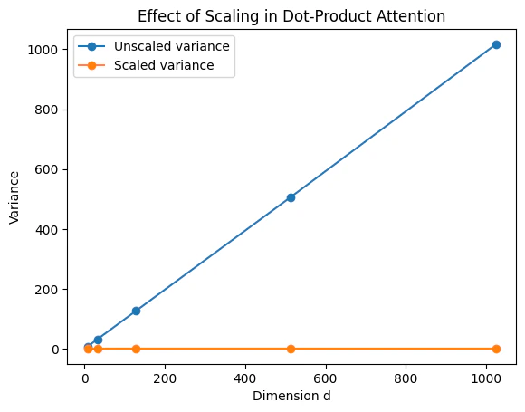
Why divide by √d?
If we define the scaled score as: Then: The variance of the attention logits is constant regardless of dimension , keeping the softmax numerically stable across different embedding sizes. Without scaling, as grows the dot product variance grows linearly, causing the softmax to become extremely sharp, one large value dominates and others vanish, leading to poor gradient flow. With scaling, the dot product distribution is normalized and the softmax stays smooth and expressive.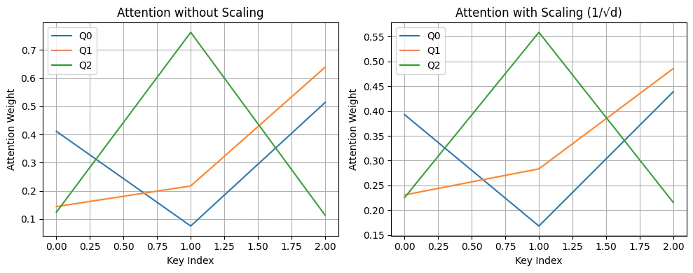
Summary
- Without scaling, attention scores can be overly large, leading to softmax outputs that are near one-hot.
- This results in vanishing gradients and unstable training.
- Scaling by normalizes the variance of the dot product, improving gradient flow and model stability.
PyTorch reference
| PyTorch class | Description |
|---|---|
nn.Linear | Applies an affine linear transformation to the incoming data: . |
nn.Softmax | Applies the Softmax function to an n-dimensional input Tensor. |
nn.MultiheadAttention | Allows the model to jointly attend to information from different representation subspaces. |