PyTorch reference
| PyTorch class | Description |
|---|---|
nn.Linear | Applies an affine linear transformation to the incoming data: . |
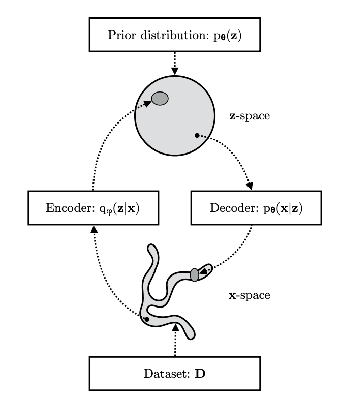
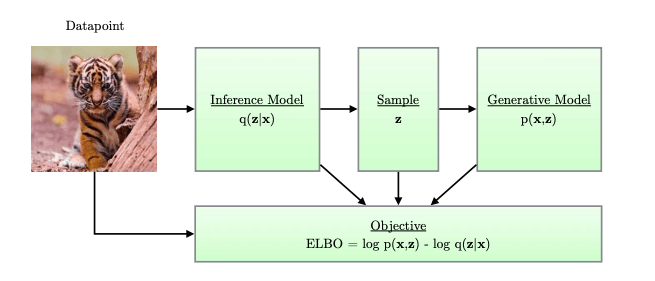
Encoder-decoder architecture with variational inference and amortized posterior approximation.
| PyTorch class | Description |
|---|---|
nn.Linear | Applies an affine linear transformation to the incoming data: . |