Velocity fields

Prerequisites. If you are unfamiliar with ODEs or the Euler integration step, first read ODEs and the Euler method. The discrete update in that section is also used here to track particles through the storm field.

A storm is a familiar example of a velocity field. Its wind has three properties:

Wind has direction.
Wind has magnitude.
Different locations experience different winds.

Mathematically, the wind in a storm forms a velocity field:

\mathbf{v}(x, y, t)

At each location

(x, y)

and time

t

, the vector gives the direction and speed of the air.

A rotating storm

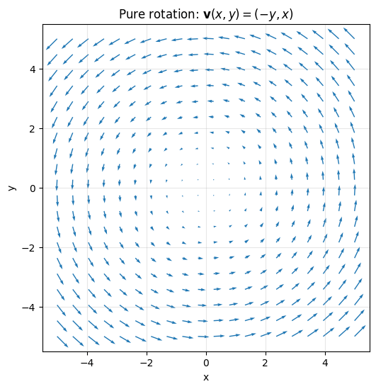
A simple 2D rotating storm centered at the origin is

\mathbf{v}(x, y) = \begin{bmatrix} -y \\ x \end{bmatrix}.

This field produces pure rotation. Its values at two points are:

At $(1, 0)$ , $\mathbf{v} = (0, 1)$ , so the wind blows upward.
At $(0, 1)$ , $\mathbf{v} = (-1, 0)$ , so the wind blows to the left.

The field therefore rotates counterclockwise around the origin.

Show plotting code

import numpy as np
import matplotlib.pyplot as plt

x = np.linspace(-5, 5, 20)
y = np.linspace(-5, 5, 20)
X, Y = np.meshgrid(x, y)

U = -Y
V = X

fig, ax = plt.subplots(figsize=(6, 6))
ax.quiver(X, Y, U, V, color="C0")
ax.set_title("Pure rotation: $\\mathbf{v}(x, y) = (-y, x)$")
ax.set_xlabel("x"); ax.set_ylabel("y")
ax.set_aspect("equal")
ax.grid(alpha=0.3)
plt.show()

Velocity weakens with distance

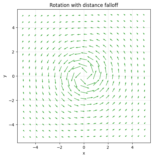
A real storm is strongest near the eye and weakens outward. A simple model for this behavior is

\mathbf{v}(x, y) = \frac{1}{x^2 + y^2 + \varepsilon} \begin{bmatrix} -y \\ x \end{bmatrix},

where

\varepsilon > 0

avoids the singularity at the origin. The field is strong near the center and decays with distance. The following plot shows this behavior.

Show plotting code

eps = 0.5
norm = X**2 + Y**2 + eps
U = -Y / norm
V = X / norm

fig, ax = plt.subplots(figsize=(6, 6))
ax.quiver(X, Y, U, V, color="C2")
ax.set_title("Rotation with distance falloff")
ax.set_xlabel("x"); ax.set_ylabel("y")
ax.set_aspect("equal")
ax.grid(alpha=0.3)
plt.show()

Particles in the storm

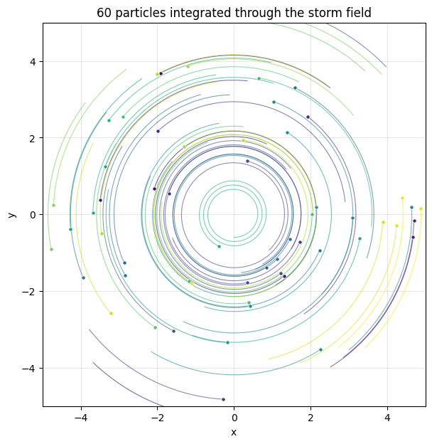
Particle motion in a velocity field is a dynamical system. A particle at position

\mathbf{x}(t)

moves according to

\frac{d \mathbf{x}}{d t} = \mathbf{v}(\mathbf{x}).

You can integrate this numerically. The simplest scheme is the Euler step,

\mathbf{x}(t + \Delta t) = \mathbf{x}(t) + \Delta t \cdot \mathbf{v}(\mathbf{x}(t)),

Repeat this update to follow many particles released at

t = 0

. The resulting trajectories model the motion of raindrops, leaves, and debris in a storm.

def storm_v(p, eps=0.5):
    x, y = p[..., 0], p[..., 1]
    norm = x**2 + y**2 + eps
    return np.stack([-y / norm, x / norm], axis=-1)


rng = np.random.default_rng(0)
n_particles = 60
n_steps = 400
dt = 0.05

particles = rng.uniform(-4, 4, size=(n_particles, 2))
trajectories = np.empty((n_steps + 1, n_particles, 2))
trajectories[0] = particles

for step in range(n_steps):
    trajectories[step + 1] = trajectories[step] + dt * storm_v(trajectories[step])

Show plotting code

fig, ax = plt.subplots(figsize=(7, 7))
colors = plt.cm.viridis(np.linspace(0, 1, n_particles))
for i in range(n_particles):
    ax.plot(trajectories[:, i, 0], trajectories[:, i, 1],
            color=colors[i], alpha=0.6, lw=0.8)
    ax.scatter(trajectories[-1, i, 0], trajectories[-1, i, 1],
               color=colors[i], s=14, zorder=3, edgecolor="white", linewidth=0.5)
ax.set_title(f"{n_particles} particles integrated through the storm field")
ax.set_xlabel("x"); ax.set_ylabel("y")
ax.set_xlim(-5, 5); ax.set_ylim(-5, 5)
ax.set_aspect("equal")
ax.grid(alpha=0.3)
plt.show()

Edit this page on GitHub or file an issue.

Latent Transport Models

Mixture of Gaussians

Variational Autoencoders

Diffusion Models

Probability Transport Models

A rotating storm

Velocity weakens with distance

Particles in the storm

​A rotating storm

​Velocity weakens with distance

​Particles in the storm

A rotating storm

Velocity weakens with distance

Particles in the storm