
Open In Colab

The transport problem

A generative model starts from a density that is easy to sample and ends at the density of the data. In this chapter the source is the standard normal p0=N(0,1)p_0 = \mathcal{N}(0, 1) on the real line. The target plays the role of the data. It is a mixture of three Gaussians, p1(x)=∑k=13πk N(x; μk,σk2),p_1(x) = \sum_{k=1}^{3} \pi_k \, \mathcal{N}(x;\, \mu_k, \sigma_k^2), with weights πk=(0.3,0.5,0.2)\pi_k = (0.3, 0.5, 0.2), means μk=(−2,1,3.5)\mu_k = (-2, 1, 3.5) and standard deviations σk=(0.4,0.6,0.3)\sigma_k = (0.4, 0.6, 0.3). Time runs from t=0t = 0, where the mass is distributed as p0p_0, to t=1t = 1, where it is distributed as p1p_1. The diffusion sections later in the book run time in the opposite direction. Three objects describe how the mass gets from p0p_0 to p1p_1. The probability path pt(x)p_t(x) says where the mass is at time tt. The velocity field vt(x)v_t(x) says which way, and how fast, the mass at position xx moves at time tt. A particle trajectory xtx_t follows one sample as the field carries it. This section is about the two endpoints and the ways of pairing them. Fields and trajectories return in the section on dynamic transport. The figure below shows one probability path. Draw x0∼p0x_0 \sim p_0 and x1∼p1x_1 \sim p_1 independently and move along the straight line xt=(1−t) x0+t x1x_t = (1 - t)\,x_0 + t\,x_1. The density of xtx_t at each time is a column of the heatmap. Time runs from left to right, and brighter color means more mass. The source density is drawn outside the left edge and the target density outside the right edge. Every transport method in this chapter is drawn in this format, so you can compare them side by side.
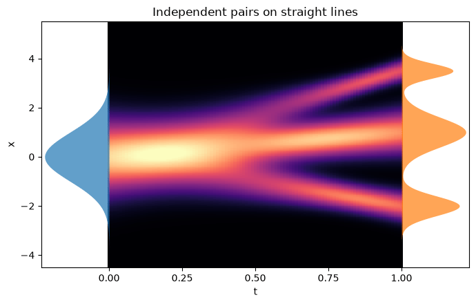
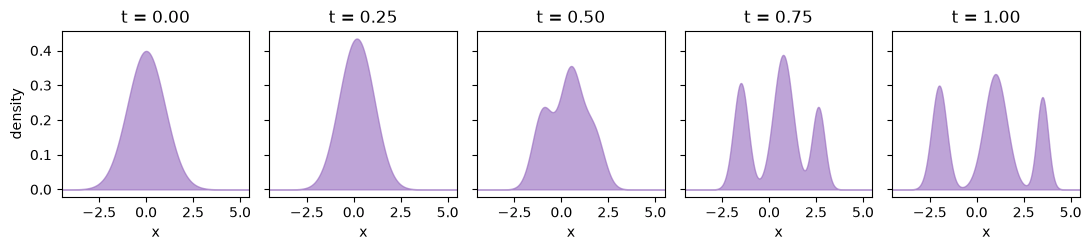
Heatmap of the probability path with time from 0 to 1 on the horizontal axis and x on the vertical axis. The standard normal source is drawn as a profile on the left edge and the three-component mixture target as a profile on the right edge. The bright band starts as one wide bump, narrows slightly before t = 0.25, and splits into three bands that end at the three target components. The probability path of independent pairs joined by straight lines. The source p0p_0 is on the left, the target p1p_1 on the right. The figure below shows the same path at five times. Five density plots of the same path at times 0, 0.25, 0.5, 0.75 and 1. At time 0 the density is a single standard normal bump. At 0.25 it is slightly narrower and taller. At 0.5 it has a main peak with two shoulders, and at 0.75 and 1 it has three separate bumps, the mixture components. Snapshots of ptp_t at five times. Each snapshot is a vertical slice of the heatmap. The single bump narrows a little before it splits. This narrowing comes from the choice of path. Another path between the same endpoints need not narrow. Four questions follow, and the sections of this chapter answer them: What shapes the intermediate density? Which other paths join the same two endpoints? Which velocity field produces each path? Which path costs the least to follow? This section starts with the last question, asked about the endpoints only: which way of pairing source points with target points is the cheapest?

Transport maps

The first answer, due to Monge, is a function that sends each source point to a target point. A map TT transports p0p_0 to p1p_1 when x0∼p0x_0 \sim p_0 gives T(x0)∼p1T(x_0) \sim p_1. This is written T♯ p0=p1,T_\sharp \, p_0 = p_1, and read as ”TT pushes p0p_0 forward to p1p_1”. In 1D such maps are easy to build from cumulative distribution functions. Write F0F_0 for the CDF of p0p_0 and F1F_1 for the CDF of p1p_1. If x0∼p0x_0 \sim p_0, then F0(x0)F_0(x_0) is uniform on (0,1)(0, 1). Applying the quantile function F1−1F_1^{-1} to a uniform variable produces a sample of p1p_1. So the increasing map T(x)=F1−1(F0(x))T(x) = F_1^{-1}\bigl(F_0(x)\bigr) transports p0p_0 to p1p_1. If UU is uniform, so is 1−U1 - U. The decreasing map F1−1(1−F0(x))F_1^{-1}\bigl(1 - F_0(x)\bigr) therefore also transports p0p_0 to p1p_1. The mixture CDF has no elementary inverse, so F1−1(u)F_1^{-1}(u) is computed by searching for the root of F1(x)=uF_1(x) = u. The largest error of this inversion over a grid of quantile levels is printed below. Both maps used in this section rely on it.
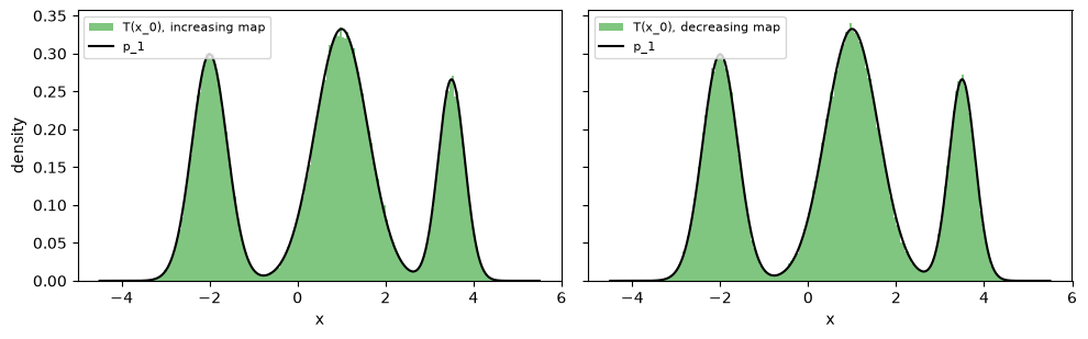
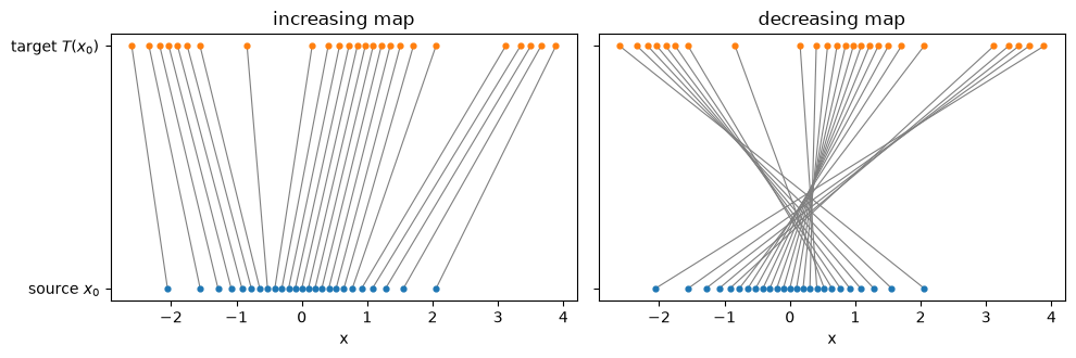
Two histograms of 200,000 transported samples, one for the increasing map and one for the decreasing map. Both histograms follow the black curve of the three-component target density closely. Histograms of T(x0)T(x_0) for 200,000 samples x0∼p0x_0 \sim p_0. Both maps reproduce p1p_1. The two maps produce the same distribution, but they pair points very differently. The schematic below draws a line from x0x_0 on the source axis to T(x0)T(x_0) on the target axis, for source points at evenly spaced quantile levels. The increasing map keeps the order of the points, so its lines never cross. The decreasing map reverses the order, so every pair of its lines crosses. Two line schematics. In each, 25 source points on a lower axis are joined by straight lines to their images on an upper axis. For the increasing map the lines fan out without crossing. For the decreasing map the leftmost source point goes to the rightmost target and every pair of lines crosses. Source points at 25 quantile levels and their images. Matching the target density does not decide which source point goes where.

Monge’s problem

Monge asked for the map with the smallest transport cost. With the squared distance as the cost of moving one unit of mass, the problem is min⁡T : T♯p0=p1  ∫(x−T(x))2 p0(x) dx.\min_{T \,:\, T_\sharp p_0 = p_1} \; \int (x - T(x))^2 \, p_0(x) \, dx . The integral is the average of (x0−T(x0))2(x_0 - T(x_0))^2 over x0∼p0x_0 \sim p_0. Two pairs of points show why the increasing map is cheaper. Take two source points a<ba < b of equal mass and two targets c<dc < d. The ordered pairing sends a→ca \to c and b→db \to d. The crossed pairing sends a→da \to d and b→cb \to c. The squares a2,b2,c2,d2a^2, b^2, c^2, d^2 cancel in the difference of the two costs, which leaves (a−d)2+(b−c)2−(a−c)2−(b−d)2=2(ac+bd−ad−bc)=2(b−a)(d−c)>0.\begin{aligned} &(a - d)^2 + (b - c)^2 - (a - c)^2 - (b - d)^2 \\ &\quad = 2(ac + bd - ad - bc) \\ &\quad = 2(b - a)(d - c) > 0 . \end{aligned} The crossed pairing always costs more. A map that is not increasing sends some pair a<ba < b to T(a)>T(b)T(a) > T(b), and swapping the targets of small intervals of mass around aa and bb lowers the cost. So in 1D the cheapest map is the increasing one, T=F1−1∘F0T = F_1^{-1} \circ F_0 (Santambrogio, 2015). For nn source points and nn target points of equal mass, the same argument says that you solve the discrete problem by sorting both lists and pairing them in order. The code below computes the cost of both maps on the mixture and checks the two-point identity on random points.
None of these checks use the particular weights, means or widths of the mixture. The code below repeats them for a second target, an equal mixture of N(−1.5,0.52)\mathcal{N}(-1.5, 0.5^2) and N(2,0.52)\mathcal{N}(2, 0.5^2). If you change PI, MU and SIGMA at the top of this section, the checks above still apply.

Couplings

A map sends each source point to exactly one place. Sometimes mass has to split. Take one source point x=0x = 0 with mass 1 and two target points y=1y = 1 and y=2y = 2 with mass 1/21/2 each. Any map sends the whole source point to a single target, so no map transports this source to this target. Kantorovich replaced maps with couplings. A coupling π\pi is a joint distribution of a pair (x,y)(x, y) whose first marginal is p0p_0 and whose second marginal is p1p_1. It says how much mass at xx goes to yy, and the mass at one xx may spread over several yy. The cost of a coupling is Eπ[(x−y)2]\mathbb{E}_{\pi}\bigl[(x - y)^2\bigr], and Kantorovich’s problem is to minimize this cost over all couplings (Santambrogio, 2015; Peyré & Cuturi, 2018). A coupling need not have a density. The coupling of a map TT puts all its mass on the graph y=T(x)y = T(x), so maps are a special case. On finitely many points a coupling is a matrix PP with Pij≥0P_{ij} \ge 0, row sums equal to the source masses aia_i and column sums equal to the target masses bjb_j. Its cost is ∑ijCijPij\sum_{ij} C_{ij} P_{ij} with Cij=(xi−yj)2C_{ij} = (x_i - y_j)^2. Both the cost and the constraints are linear in PP, so the problem is a linear program. For the split example the only coupling sends half of the mass to each target, and the solver finds it.
Between two densities on the line a map always exists. Couplings still give more ways to pair points than maps do. The simplest is the independent coupling p0⊗p1p_0 \otimes p_1, which draws xx and yy separately. It is the coupling behind the path at the top of this section. Expanding the square and using E[x]=0\mathbb{E}[x] = 0 and E[x2]=1\mathbb{E}[x^2] = 1 for the standard normal gives its cost, E[(x−y)2]=1+Ep1[y2]=1+∑kπk(μk2+σk2).\begin{aligned} \mathbb{E}\bigl[(x - y)^2\bigr] &= 1 + \mathbb{E}_{p_1}\bigl[y^2\bigr] \\ &= 1 + \sum_k \pi_k \bigl(\mu_k^2 + \sigma_k^2\bigr). \end{aligned} The code below compares this formula with a sampled estimate.
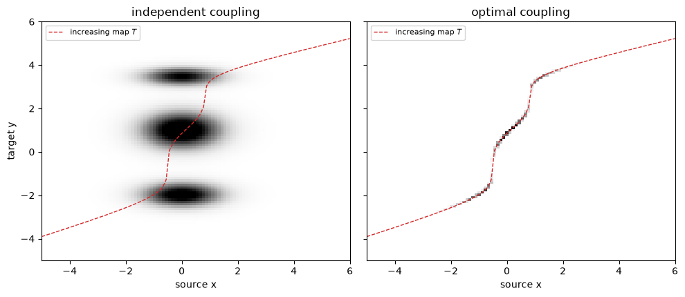
To find the optimal coupling of the two densities, put both on a grid of nn points over [−5,6][-5, 6], give each grid point the mass of its density value (normalized to sum to 1), and solve the linear program. The figure shows the result for n=100n = 100 next to the independent coupling. Each panel is the matrix PP, with source position on the horizontal axis and target position on the vertical axis.
Two coupling matrices on a 100-point grid, source position on the horizontal axis and target position on the vertical axis. The independent coupling is three horizontal blobs, one per target component, each spread over source positions from about -2 to 2. The optimal coupling is a thin increasing staircase curve lying on the dashed red graph of the increasing map. Left, the independent coupling spreads each source point over the whole target. Right, the optimal coupling from the linear program concentrates on the graph of the increasing map TT (dashed). The optimal coupling of the grid problem is the coupling of the increasing map, up to the resolution of the grid. On the line, then, Kantorovich’s problem and Monge’s problem have the same answer. Couplings matter in this chapter for another reason: the flow matching section trains on pairs (x0,x1)(x_0, x_1) drawn from a coupling, and the choice of coupling shapes the path it learns.

The Wasserstein distance

The cost of the optimal coupling is the squared Wasserstein distance, W22(p0,p1)=min⁡π  Eπ[(x−y)2],W_2^2(p_0, p_1) = \min_{\pi} \; \mathbb{E}_{\pi}\bigl[(x - y)^2\bigr], where the minimum runs over all couplings of p0p_0 and p1p_1. In 1D the optimal coupling pairs equal quantile levels: the point at level uu of p0p_0 goes to the point at level uu of p1p_1. Substituting u=F0(x)u = F_0(x) in the cost of the increasing map gives W22(p0,p1)=∫01(F0−1(u)−F1−1(u))2 du,W_2^2(p_0, p_1) = \int_0^1 \bigl(F_0^{-1}(u) - F_1^{-1}(u)\bigr)^2 \, du , the squared L2L^2 distance between the two quantile functions (Peyré & Cuturi, 2018). The code below evaluates this integral and compares it with the linear program as the grid is refined.
The relative error of the grid answer falls from about 0.9% at n=50n = 50 to about 0.05% at n=200n = 200. The quantile formula also agrees with the sampled cost of the increasing map from Monge’s problem, to the third decimal place. W2W_2 is a distance between densities. It is zero only when the two densities are equal, it is symmetric, and it satisfies the triangle inequality. Its value is the cost of moving one density into the other, so it compares densities by how far their mass must travel. Two narrow bumps that do not overlap are far apart in W2W_2 when their centers are far apart and close when their centers are close. A measure that compares density values point by point, such as the total variation distance, gives the same value in both cases, because the bumps never overlap. Later sections compare the kinetic action of every path with W22W_2^2.

Optional: entropic transport and Sinkhorn iterations

This subsection is outside the main line of the chapter. You can skip to Brenier’s theorem below. The linear program grows quickly with the number of points: a grid of nn points has n2n^2 unknowns. Cuturi’s remedy was to add an entropy term to the cost (Cuturi, 2013). For ε>0\varepsilon > 0, solve min⁡P  ∑ijCijPij−εH(P),H(P)=−∑ijPij(log⁡Pij−1),\begin{aligned} &\min_{P} \; \sum_{ij} C_{ij} P_{ij} - \varepsilon H(P), \\ &H(P) = -\sum_{ij} P_{ij} \bigl(\log P_{ij} - 1\bigr), \end{aligned} over the same matrices PP with row sums aa and column sums bb. The solution has the form Pij=uiKijvjP_{ij} = u_i K_{ij} v_j with Kij=e−Cij/εK_{ij} = e^{-C_{ij}/\varepsilon}. Sinkhorn’s algorithm finds the scalings by alternating between the two marginal constraints: u←a⊘(Kv),v←b⊘(K⊤u),u \leftarrow a \oslash (K v), \qquad v \leftarrow b \oslash (K^\top u), where ⊘\oslash divides entry by entry. For small ε\varepsilon the entries of KK underflow, so the iteration below runs on the logarithms of the scalings.
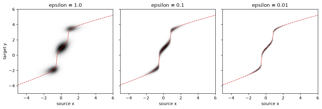
Three entropic coupling matrices for epsilon 1, 0.1 and 0.01 on the same axes as the linear program figure. At epsilon 1 the mass is three blurred blobs around the dashed increasing map. At 0.1 the band is narrower, and at 0.01 it is a thin curve on the dashed line. Entropic couplings for three values of ε\varepsilon. The dashed line is the increasing map. A large ε\varepsilon rewards spread, so the coupling blurs toward the independent coupling and its cost rises. As ε\varepsilon shrinks, the coupling and its cost approach the linear program. Each Sinkhorn iteration is two matrix-vector products, which run in parallel on modern hardware, and the result is a differentiable function of the masses and the costs. Because of these two properties, entropic transport can be computed at scale and used inside a training loss.

Brenier’s theorem

In more than one dimension there is no ordering to sort by, but the answer has the same structure. For the squared distance cost and a source p0p_0 with a density, Brenier’s theorem states that the optimal coupling is given by a map, that this map is unique, and that it is the gradient of a convex function (Santambrogio, 2015; Peyré & Cuturi, 2018). In 1D an increasing function is the derivative of a convex function, so the quantile map F1−1∘F0F_1^{-1} \circ F_0 is the Brenier map of this section. In higher dimensions the theorem guarantees the map but gives no formula for it, and it has to be computed numerically. Key references: (Peyré & Cuturi, 2018; Santambrogio, 2015; Cuturi, 2013)

References

  • Cuturi, M. (2013). Sinkhorn Distances: Lightspeed Computation of Optimal Transportation Distances. arXiv [stat.ML]. DOI
  • Peyré, G., Cuturi, M. (2018). Computational Optimal Transport. arXiv [stat.ML]. DOI
  • Santambrogio, F. (2015). Optimal transport for applied mathematicians – calculus of variations, PDEs and modeling.

Found an error on this page? Report an issue.