Open In Colab

Learning the field from samples

The dynamic transport section moved the standard normal p0p_0 to the mixture p1p_1 along the geodesic, and it could compute everything exactly: the density ptp_t, its CDF FtF_t and the field vtv_t. Two facts from that section carry over. A field vtv_t moves a path ptp_t when the pair satisfies the continuity equation ∂tpt+∂x(ptvt)=0\partial_t p_t + \partial_x (p_t v_t) = 0. In 1D the path fixes the field, vt(x)=−∂tFt(x)/pt(x)v_t(x) = -\partial_t F_t(x) / p_t(x). All of this was possible because the mixture was built by hand, so its density and CDF are known. For real data such as images you have samples of p1p_1 and nothing else: no density, no CDF, no field. Flow matching learns a field from samples alone (Lipman et al., 2022). The general definitions are on the flow matching page. This section runs flow matching on the same mixture, where every learned quantity can still be compared with an exact reference. The code below repeats the grids and the geodesic functions of the dynamic transport section.

A path you can sample

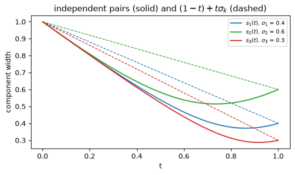
Flow matching builds its path from pairs. Draw x0∼p0x_0 \sim p_0 and x1∼p1x_1 \sim p_1 independently and move along the segment between them, xt=(1−t) x0+t x1.x_t = (1 - t)\,x_0 + t\,x_1 . Samples of this path cost nothing: draw a pair and a time. The density is also known for the mixture. Given that x1x_1 comes from component kk, xtx_t is a sum of two independent Gaussians, so it is Gaussian with mean tμkt\mu_k and variance sk2(t)=(1−t)2+t2σk2.s_k^2(t) = (1 - t)^2 + t^2 \sigma_k^2 . So ptp_t is again a mixture, with the same weights πk\pi_k, means tμkt\mu_k and widths sk(t)s_k(t). Its CDF is the same mixture of normal CDFs. Compare the width with the geodesic between N(0,1)\mathcal{N}(0, 1) and a single component N(μk,σk2)\mathcal{N}(\mu_k, \sigma_k^2). There the width interpolates in a straight line, (1−t)+tσk(1 - t) + t\sigma_k. The independent path is narrower at every time in between. Each component shrinks below its final width σk\sigma_k and then widens to σk\sigma_k at t=1t = 1.
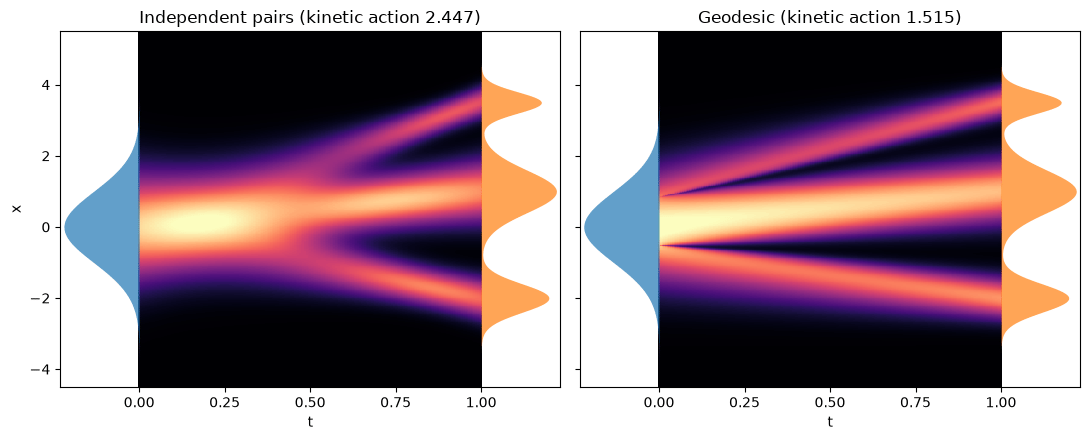
Line plot of component width against t for the three mixture components. Solid curves for the independent-pair path start at 1, fall below their final widths 0.4, 0.6 and 0.3, and rise back to them at t = 1. Dashed straight lines from 1 to each final width lie above the solid curves at every interior time. Width of each mixture component along the independent-pair path (solid) and along the straight interpolation of widths (dashed). Each solid curve falls below its final value before it returns to it at t=1t = 1. The standard figure puts the independent-pair path next to the geodesic. The field of each path comes from the 1D formula of the dynamic transport section, and the title of each panel reports its kinetic action.
Two standard transport heatmaps side by side. Left, the independent-pair path, with kinetic action 2.447: the source bump narrows until about t = 0.3 and splits into three bands after t = 0.5. Right, the geodesic, with kinetic action 1.515: the bump splits into three straight bands right at t = 0. Left, the independent-pair path of flow matching. Right, the geodesic of the dynamic transport section. Both join the same endpoints. The independent-pair path keeps p0p_0 in one piece for longer. It narrows first and splits into the three components late. The geodesic splits right away. The independent path also costs more, and the last subsections measure by how much.

Conditional paths and the marginal field

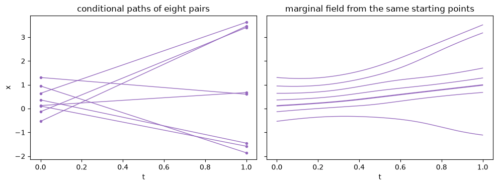
Each pair moves along its own straight line with constant velocity x1−x0x_1 - x_0. These conditional paths cross: a pair that starts low can end high, and another pair can do the opposite. At a crossing point two lines pass through the same xx at the same tt with different velocities. A field assigns one velocity to each point, so it cannot follow both lines. The field of the path averages the velocities of all pairs that pass through xx at time tt, vt(x)=E[X1−X0∣Xt=x].v_t(x) = \mathbb{E}\bigl[X_1 - X_0 \mid X_t = x\bigr] . This is the marginal field. Its trajectories never cross, because two solutions of x˙=vt(x)\dot x = v_t(x) that meet at some time are the same trajectory. For the mixture the average has a closed form. Given component kk, XtX_t and X1−X0X_1 - X_0 are jointly Gaussian with covariance tσk2−(1−t)=sks˙kt\sigma_k^2 - (1 - t) = s_k \dot s_k, and conditioning a Gaussian gives a linear function of xx. Averaging over the components gives vt(x)=∑kwk(x,t) uk(x,t),uk(x,t)=μk+s˙k(t)sk(t) (x−tμk),\begin{aligned} v_t(x) &= \sum_k w_k(x, t)\, u_k(x, t), \\ u_k(x, t) &= \mu_k + \frac{\dot s_k(t)}{s_k(t)}\,(x - t\mu_k), \end{aligned} where s˙k=(tσk2−(1−t))/sk\dot s_k = (t\sigma_k^2 - (1 - t))/s_k and wk(x,t)w_k(x, t) is the responsibility of component kk at xx: its share πk N(x;tμk,sk2)/pt(x)\pi_k\, \mathcal{N}(x; t\mu_k, s_k^2) / p_t(x) of the density there. The code below implements this field and an integrator for particle trajectories. It then compares the field with the 1D formula, on the grid points where pt(x)>10−3p_t(x) > 10^{-3} as in the dynamic transport section.
The two computations agree to better than 10−410^{-4}. The figure below shows eight pairs drawn independently. On the left each pair moves along its straight conditional path. On the right the same eight starting points follow the marginal field.
Two panels of eight trajectories. Left, straight lines joining eight independent pairs from t = 0 to t = 1; several lines cross each other. Right, the marginal-field trajectories from the same eight starting points; they curve, keep their order and never cross. Left, eight independent pairs joined by straight lines; several lines cross. Right, the trajectories of the marginal field from the same eight starting points. They keep their order and bend instead of crossing.

Particles carry the density

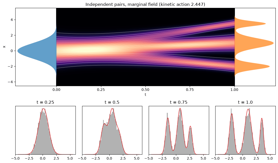
The marginal field moves the path: integrating x˙=vt(x)\dot x = v_t(x) from samples of p0p_0 gives samples of ptp_t at every tt. The code below integrates 4000 samples of p0p_0 with an accurate solver and compares them at several times with the exact ptp_t. The comparison uses the Kolmogorov-Smirnov (KS) distance, the largest gap between the empirical CDF of the particles and FtF_t.
Top, the standard heatmap of the independent-pair path with 40 white trajectories of the marginal field that stay together, then fan out into three bands. Bottom, four histograms of 4000 particles at t = 0.25, 0.5, 0.75 and 1, each matching the red exact density, which goes from one bump to three. Top, the standard figure of the independent-pair path with 40 trajectories of the marginal field. Bottom, histograms of all 4000 particles at four times, with the exact ptp_t in red. At every time the KS distance equals the distance of the 4000 starting samples to p0p_0, to three decimal places. The flow keeps the order of the particles and moves p0p_0 to ptp_t, so the particle at quantile level uu goes to Ft−1(u)F_t^{-1}(u), and the empirical CDF keeps its shape. What remains is the sampling error of the initial draw. The same value serves later as the floor for judging learned fields.

The loss is least squares

For a sample xtx_t you can compute the velocity x1−x0x_1 - x_0 of its own pair, but not the marginal field vt(xt)v_t(x_t), which averages over all pairs. Flow matching uses a fact about regression. For random variables XX and YY, the function that minimizes E[(Y−f(X))2]\mathbb{E}\bigl[(Y - f(X))^2\bigr] is the conditional mean f⋆(x)=E[Y∣X=x]f^\star(x) = \mathbb{E}[Y \mid X = x]. Take the input to be (Xt,t)(X_t, t), with tt uniform on [0,1][0, 1], and the target to be Y=X1−X0Y = X_1 - X_0. The minimizer is the marginal field. So you can train a network vθ(x,t)v_\theta(x, t) on the loss L(θ)=E[(vθ(Xt,t)−(X1−X0))2],L(\theta) = \mathbb{E}\Bigl[\bigl(v_\theta(X_t, t) - (X_1 - X_0)\bigr)^2\Bigr], with per-pair targets you can always compute (Lipman et al., 2022; Yaron et al., 2024). The loss does not go to zero. Its smallest value is the variance of the target around its conditional mean, which is Lmin⁡=E[(X1−X0)2]−∫01E[vt(Xt)2] dt=1+Ep1[X12]−A,\begin{aligned} L_{\min} &= \mathbb{E}\bigl[(X_1 - X_0)^2\bigr] - \int_0^1 \mathbb{E}\bigl[v_t(X_t)^2\bigr]\,dt \\ &= 1 + \mathbb{E}_{p_1}\bigl[X_1^2\bigr] - A , \end{aligned} where AA is the kinetic action of the path. The code below defines a network with two hidden layers of 64 units, trains it for 10,000 steps on batches of 4096 independent pairs, and prints the training time.
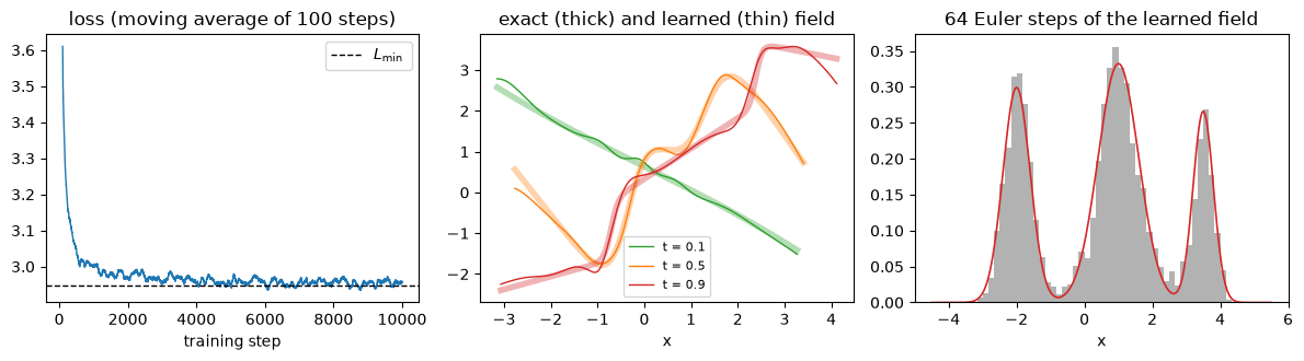
Three panels. Left, the training loss falls quickly from about 3.6 and levels off just above a dashed line at the smallest possible loss near 2.95. Middle, learned and exact fields at t = 0.1, 0.5 and 0.9 nearly overlap, with small deviations at the edges. Right, a histogram of samples after 64 Euler steps matching the red three-component target density. Left, the training loss with the smallest possible loss Lmin⁡L_{\min} (dashed). Middle, the learned field and the exact marginal field at three times, drawn where pt>10−3p_t > 10^{-3}. Right, the 4000 samples moved by 64 Euler steps of the learned field, against p1p_1 in red. The loss levels off within 2% of Lmin⁡L_{\min}, and the remaining spread is the noise in the per-pair targets. Because the floor is far from zero, the value of the loss does not show how close the learned field is to the exact one. The middle panel compares the two fields directly, and the last subsection measures the error.

Same endpoint, different path

The marginal field keeps the order of particles, so its endpoint map x0↦x1x_0 \mapsto x_1 is increasing. An increasing map that moves p0p_0 to p1p_1 is unique on the line: it is the Monge map T=F1−1∘F0T = F_1^{-1} \circ F_0 of the first section. The flow of independent pairs therefore ends where optimal transport ends. The code below checks this on the 4000 samples, for ∣x0∣<2.5|x_0| < 2.5, and computes the kinetic action of the path.
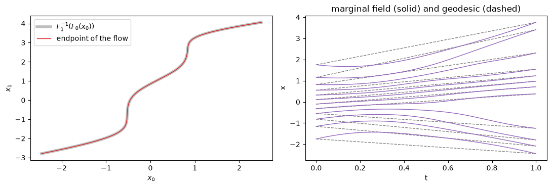
Two panels. Left, the endpoint of the flow plotted against the starting point lies exactly on the Monge map curve, which rises steeply near x0 = -0.5 and x0 = 0.8. Right, twelve curved trajectories of the marginal field next to dashed straight geodesic lines from the same starting points to the same endpoints. Left, the endpoint of the flow against the Monge map; the two curves coincide. Right, twelve trajectories of the marginal field and the straight geodesic lines from the same starting points. Each pair of curves shares its endpoints. The endpoints agree to about 10−710^{-7}, but the paths differ. The flow trajectories bend, while the geodesic moves each point in a straight line at constant speed, and the kinetic action of the independent-pair path is more than one and a half times W22W_2^2. By the Benamou-Brenier formula no path costs less than W22W_2^2, and the independent-pair path is not the minimizer. The endpoints agree only because the example is 1D, where an increasing transport map is unique. In two or more dimensions the flow of independent pairs moves p0p_0 to p1p_1, but its endpoint map is in general not the optimal transport map.

Three couplings

Flow matching does not require independent pairs. Any joint distribution of (x0,x1)(x_0, x_1) with marginals p0p_0 and p1p_1, any coupling in the sense of the first section, gives a path whose time-1 density is p1p_1. The regression recipe is unchanged. Three couplings are compared here.
  1. Independent pairs, as above.
  2. The quantile coupling. Draw UU uniform on (0,1)(0, 1) and set x0=F0−1(U)x_0 = F_0^{-1}(U) and x1=F1−1(U)x_1 = F_1^{-1}(U). This is the optimal coupling of the first section. Its conditional paths are the straight lines of the geodesic, and they never cross, so the marginal field is the geodesic field and the regression target has no noise. This coupling is the reference.
  3. Sorted minibatches. Draw a batch of independent pairs, sort the x0x_0 values and the x1x_1 values, and pair them in order. This is the optimal coupling of the two batches, not of the two densities, so it only approximates the quantile coupling, even in 1D. It needs nothing but samples, which is why minibatch optimal transport uses it when the densities are unknown (Tong et al., 2023).
Rectified flow straightens paths another way. It re-pairs each source point with the endpoint of its own learned flow and trains again (Liu et al., 2022). The code below trains a network on each of the other two couplings with the same settings.
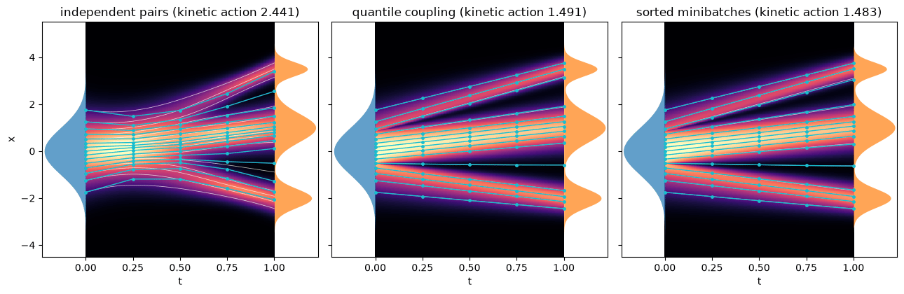
Each learned field is compared with its exact field, weighted by the density of the path: the relative error e=(∑t,xpt(x) (vθ(x,t)−vt(x))2∑t,xpt(x) vt(x)2)1/2e = \left(\frac{\sum_{t, x} p_t(x)\,\bigl(v_\theta(x, t) - v_t(x)\bigr)^2}{\sum_{t, x} p_t(x)\, v_t(x)^2}\right)^{1/2} over the grid. For independent pairs vtv_t is the closed-form field. For the quantile coupling it is the geodesic field. The sorted coupling has no closed form, and its error is measured against the geodesic field, which it approximates. This error is the training error, except for the sorted coupling, where it also includes the bias of pairing within batches. The kinetic action of each learned field is the average of ∫01vθ(xt,t)2 dt\int_0^1 v_\theta(x_t, t)^2\,dt over trajectories from the 4000 samples, computed with an accurate solver. It is compared with W22W_2^2 and with ArefA_{\text{ref}}, the average of (T(x0)−x0)2(T(x_0) - x_0)^2 over the same 4000 samples, which is the action of the geodesic estimated on those samples. The integration error is the root mean square distance between the endpoints after 4, 8, 16 and 64 Euler steps and the endpoints of an accurate solve. Both use the same learned field, so this distance contains no training error. The KS distance of the samples to p1p_1 measures sample quality. It mixes training error, integration error and the sampling error of the 4000 starting points, so it is reported but not used to separate the two kinds of error.
Three standard heatmaps with trajectories from 15 starting points. Left, independent pairs, kinetic action 2.441: white accurate trajectories bend, and the cyan four-step Euler polylines drift away from them. Middle, quantile coupling, action 1.491, and right, sorted minibatches, action 1.483: trajectories are straight lines and the cyan Euler points lie on them. Trajectories of the three learned fields from 15 starting points: accurate solve in white, four Euler steps in cyan. The background is the exact path density: the independent-pair path on the left, the geodesic in the middle and on the right. The sorted coupling has no closed-form path, so its panel shows the geodesic it approximates. Each title reports the kinetic action of the learned field. The first table holds the training error, in the field error column. The quantile field is learned more accurately than the independent one, because its regression target equals the field exactly. The independent target is a noisy sample around the field. With the accurate solver all three fields put their samples on p1p_1, with KS distances close to that of the exact map on the same samples. The second table holds the integration error. With four steps the endpoints of the independent coupling are far from the accurate ones, while the quantile and sorted errors are less than a fifth as large. Their trajectories are almost straight lines, and Euler steps follow a straight line without error. The independent trajectories bend, and a few straight steps cut the corners. For every coupling the error roughly halves each time the number of steps doubles, as expected of a first-order method. The KS distances in the third table follow the same order at four steps, but at 64 steps they sit near the sampling floor and no longer rank the couplings. The quantile and sorted fields have kinetic actions within a few percent of W22W_2^2, and the independent field has about the action of its exact path. The quantile and sorted actions print slightly below W22W_2^2, which no path can beat. The cause is the finite sample: the actions are averages over 4000 starting points, and on those points the geodesic itself averages ArefA_{\text{ref}}, which is below W22W_2^2. Against ArefA_{\text{ref}} the quantile action agrees to within 1%. Everything here is 1D. In more dimensions the quantile coupling has no simple form, and sorting is replaced by solving an optimal transport problem on each batch. The batch coupling then approximates the optimal one only roughly, so minibatch paths are straighter than independent ones but in general not straight (Tong et al., 2023). Key references: (Lipman et al., 2022; Yaron et al., 2024; Tong et al., 2023; Liu et al., 2022)

References

  • Lipman, Y., Chen, R., Ben-Hamu, H., Nickel, M., Le, M. (2022). Flow Matching for generative modeling. arXiv [cs.LG]. Link
  • Liu, X., Gong, C., Liu, Q. (2022). Flow straight and fast: Learning to generate and transfer data with rectified flow. arXiv [cs.LG]. DOI
  • Tong, A., Fatras, K., Malkin, N., Huguet, G., Zhang, Y., et al. (2023). Improving and generalizing flow-based generative models with minibatch optimal transport. arXiv [cs.LG]. DOI
  • Yaron, L., Marton, H., Peter, H., Neta, S., Matt, L., et al. (2024). Flow Matching Guide and Code. arXiv [cs.LG]. Link

Found an error on this page? Report an issue.