
Paths with the same endpoints
The transport maps and couplings section found the cheapest way to pair source points with target points. For the squared distance on the line it is the increasing map , and its cost is . This section asks the next question: how should the mass move through time? A map gives the endpoint of each point and says nothing about the times in between. Every path of the form starts at and ends at . The function is a schedule. With every point moves at constant speed. With every point starts slowly and speeds up. For increasing , all these paths move each point along the same segment, but at different times, so their intermediate densities differ. The code below sets up the grids used in the rest of this section: 201 times in and 2001 positions in .The fluid picture
Think of as the density of a fluid on the line and of as the velocity of the fluid at position and time . This is the picture of the storm in the velocity fields section, where the wind carries raindrops. Here the field carries probability mass. A particle at at time moves with velocity , so its trajectory solves . Probability mass is conserved: it is neither created nor destroyed. The total stays equal to 1, and mass that leaves one place must arrive somewhere next to it. The wind in the storm example did not have to conserve anything it carried.The continuity equation
Conservation of mass becomes an equation once you count the mass in a fixed interval , Mass enters or leaves the interval only through its two ends. The rate at which mass crosses a point from left to right is the flux , the density times the velocity. Mass flows in at and out at , so The second line is the fundamental theorem of calculus. Differentiating under the integral sign also gives . The two integrals agree for every interval, so their integrands agree at every point: This is the continuity equation (Santambrogio, 2015). It links a path to a field: the field moves the path when the pair satisfies it. The diffusion sections later in the book add a second flux term, for mass that spreads by random motion.Speed and kinetic energy
On the paths above, a particle moves with velocity . The kinetic action of a path is the average squared speed of its particles, integrated over time. For these paths it factors: The last step uses the result of the maps and couplings section: the cost of the increasing map is . By the Cauchy-Schwarz inequality, with equality only when is constant, that is, when . For the integral is , so this schedule costs a third more than constant speed. Of all the ways of following the map , constant speed has the smallest kinetic action, and that action is . The code below evaluates both actions.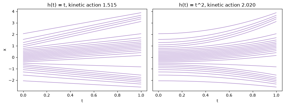
Displacement interpolation
The constant-speed paths define a probability path. The geodesic is the density of This path is called displacement interpolation (Santambrogio, 2015). Each particle moves from its own position to its target. The path is never a weighted average of and . The last part of this section computes the cost of such an average. The map is increasing, so the change of variables formula gives the density, The formula for comes from differentiating . Because the map keeps the order of points, the CDF follows too: . Each particle also moves at the constant velocity , so the field at is that velocity for the source point that reaches at time . The code below computes all three by pushing a fine grid of source points forward.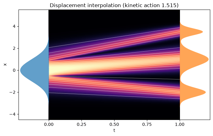
A density path fixes its field
In 1D the continuity equation can be solved for the field. Integrate it over . The first term gives , the time derivative of the CDF. The second gives , provided the flux vanishes at . So , and The path alone determines the field. The code below computes the geodesic field in two ways: from this formula, with a finite difference in , and from the particle velocities . The formula divides by , so the comparison uses only the grid points where . Farther out in the tails the field moves almost no mass, and dividing by a tiny density amplifies small numerical errors.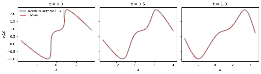
The Benamou-Brenier formula
Benamou and Brenier recast the static problem of the maps and couplings section as a problem about motion (Benamou & Brenier, 2000; Peyré & Cuturi, 2018). Consider every pair that satisfies the continuity equation, with equal to at and to at . The smallest kinetic energy among them is : The inner integral is the average squared speed of the mass at time , the same quantity as in the kinetic action. The minimizer is the geodesic. Its computed energy above matches , and the schedules showed that following the same map at uneven speed costs more. As a second check, take a path of a different kind. The mixture path blends the two densities, Its field comes from the 1D formula. Its particles follow from the same formula: along a trajectory, , so a particle keeps its quantile level and . The code below computes the field, the particles and the kinetic energy of the mixture path.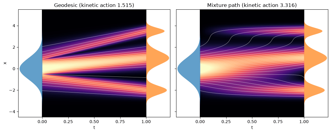
From the geodesic to flow matching
Flow matching works with the same objects: a probability path, the field that moves it, and the continuity equation that links them. It picks a path that is easy to sample and to learn from samples, and that path is not in general the geodesic. The flow matching section states the method in general, and the 1D mixture section runs it on this mixture and measures its kinetic action against . Key references: (Benamou & Brenier, 2000; Santambrogio, 2015; Peyré & Cuturi, 2018)References
- Benamou, J., Brenier, Y. (2000). A computational fluid mechanics solution to the Monge-Kantorovich mass transfer problem. Numer. Math. (Heidelb.). DOI
- Peyré, G., Cuturi, M. (2018). Computational Optimal Transport. arXiv [stat.ML]. DOI
- Santambrogio, F. (2015). Optimal transport for applied mathematicians – calculus of variations, PDEs and modeling.
Found an error on this page? Report an issue.