

Learning the field from samples
The dynamic transport section moved the standard normal to the mixture along the geodesic, and it could compute everything exactly: the density , its CDF and the field . Two facts from that section carry over. A field moves a path when the pair satisfies the continuity equation . In 1D the path fixes the field, . All of this was possible because the mixture was built by hand, so its density and CDF are known. For real data such as images you have samples of and nothing else: no density, no CDF, no field. Flow matching learns a field from samples alone (Lipman et al., 2022). The general definitions are on the flow matching page. This section runs flow matching on the same mixture, where every learned quantity can still be compared with an exact reference. The code below repeats the grids and the geodesic functions of the dynamic transport section.A path you can sample
Flow matching builds its path from pairs. Draw and independently and move along the segment between them, Samples of this path cost nothing: draw a pair and a time. The density is also known for the mixture. Given that comes from component , is a sum of two independent Gaussians, so it is Gaussian with mean and variance So is again a mixture, with the same weights , means and widths . Its CDF is the same mixture of normal CDFs. Compare the width with the geodesic between and a single component . There the width interpolates in a straight line, . The independent path is narrower at every time in between. Each component shrinks below its final width and then widens to at .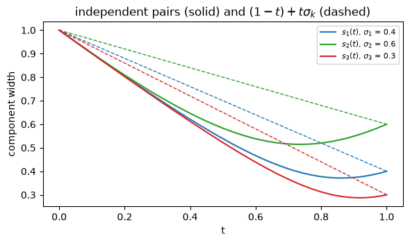
Conditional paths and the marginal field
Each pair moves along its own straight line with constant velocity . These conditional paths cross: a pair that starts low can end high, and another pair can do the opposite. At a crossing point two lines pass through the same at the same with different velocities. A field assigns one velocity to each point, so it cannot follow both lines. The field of the path averages the velocities of all pairs that pass through at time , This is the marginal field. Its trajectories never cross, because two solutions of that meet at some time are the same trajectory. For the mixture the average has a closed form. Given component , and are jointly Gaussian with covariance , and conditioning a Gaussian gives a linear function of . Averaging over the components gives where and is the responsibility of component at : its share of the density there. The code below implements this field and an integrator for particle trajectories. It then compares the field with the 1D formula, on the grid points where as in the dynamic transport section.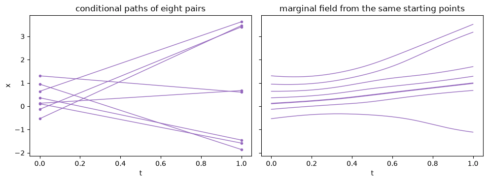
Particles carry the density
The marginal field moves the path: integrating from samples of gives samples of at every . The code below integrates 4000 samples of with an accurate solver and compares them at several times with the exact . The comparison uses the Kolmogorov-Smirnov (KS) distance, the largest gap between the empirical CDF of the particles and .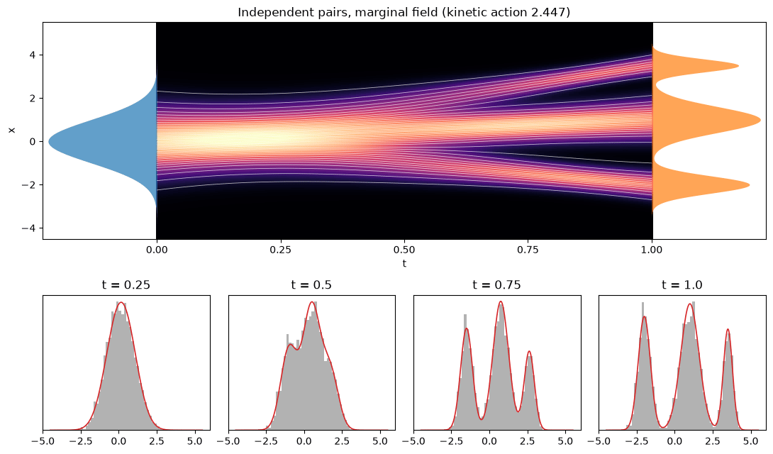
The loss is least squares
For a sample you can compute the velocity of its own pair, but not the marginal field , which averages over all pairs. Flow matching uses a fact about regression. For random variables and , the function that minimizes is the conditional mean . Take the input to be , with uniform on , and the target to be . The minimizer is the marginal field. So you can train a network on the loss with per-pair targets you can always compute (Lipman et al., 2022; Yaron et al., 2024). The loss does not go to zero. Its smallest value is the variance of the target around its conditional mean, which is where is the kinetic action of the path. The code below defines a network with two hidden layers of 64 units, trains it for 10,000 steps on batches of 4096 independent pairs, and prints the training time.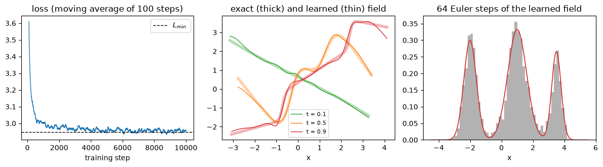
Same endpoint, different path
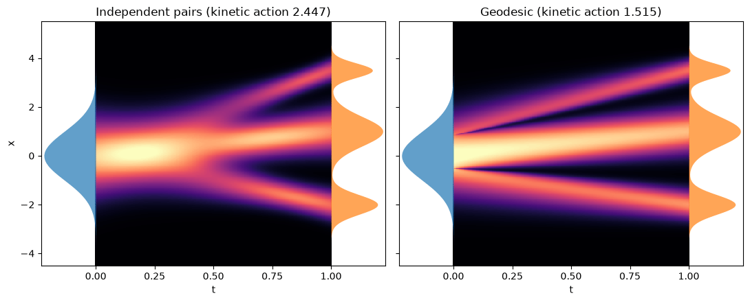
The marginal field keeps the order of particles, so its endpoint map is increasing. An increasing map that moves to is unique on the line: it is the Monge map of the first section. The flow of independent pairs therefore ends where optimal transport ends. The code below checks this on the 4000 samples, for , and computes the kinetic action of the path.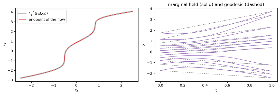
Three couplings
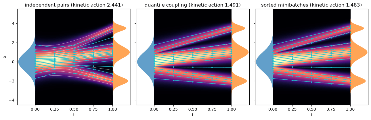
Flow matching does not require independent pairs. Any joint distribution of with marginals and , any coupling in the sense of the first section, gives a path whose time-1 density is . The regression recipe is unchanged. Three couplings are compared here.- Independent pairs, as above.
- The quantile coupling. Draw uniform on and set and . This is the optimal coupling of the first section. Its conditional paths are the straight lines of the geodesic, and they never cross, so the marginal field is the geodesic field and the regression target has no noise. This coupling is the reference.
- Sorted minibatches. Draw a batch of independent pairs, sort the values and the values, and pair them in order. This is the optimal coupling of the two batches, not of the two densities, so it only approximates the quantile coupling, even in 1D. It needs nothing but samples, which is why minibatch optimal transport uses it when the densities are unknown (Tong et al., 2023).
References
- Lipman, Y., Chen, R., Ben-Hamu, H., Nickel, M., Le, M. (2022). Flow Matching for generative modeling. arXiv [cs.LG]. Link
- Liu, X., Gong, C., Liu, Q. (2022). Flow straight and fast: Learning to generate and transfer data with rectified flow. arXiv [cs.LG]. DOI
- Tong, A., Fatras, K., Malkin, N., Huguet, G., Zhang, Y., et al. (2023). Improving and generalizing flow-based generative models with minibatch optimal transport. arXiv [cs.LG]. DOI
- Yaron, L., Marton, H., Peter, H., Neta, S., Matt, L., et al. (2024). Flow Matching Guide and Code. arXiv [cs.LG]. Link
Found an error on this page? Report an issue.