Measuring Change with Image Derivatives

This section was written by Kaushik Kachireddy (pull request #77), with help from an AI coding agent (Claude Code) on the code. It reproduces the ideas of Chapter 18 of Foundations of Computer Vision by Antonio Torralba, Phillip Isola, and William T. Freeman. The book’s own figures are not reproduced here, because the book’s license covers only the work in full; links point to them instead. The image derivative is the workhorse of low-level vision: it turns intensity changes into signals you can measure. This section builds the derivative operators of the book’s chapter: the two-tap

[1,-1]

and centered

[1,0,-1]

kernels, Gaussian derivatives (through Hermite polynomials), derivative-of-binomial kernels, the Roberts and Sobel operators, the Laplacian and Laplacian-of-Gaussian, unsharp masking, and a working Retinex decomposition. Each comes with a numerical check. The book demonstrates these operators on its own photographs. Here they run on scikit-image test images and on synthetic patterns, with a link to each of the book’s figures. Following the book, derivative maps are shown signed around mid-gray, per channel, so color inputs show colored edges.

import numpy as np
import torch
import torch.nn.functional as F
import matplotlib.pyplot as plt
from numpy.polynomial.hermite import hermval
from skimage import data, img_as_float

_ = torch.manual_seed(0); np.random.seed(0)
torch.set_default_dtype(torch.float32)
plt.rcParams.update({'figure.dpi': 130, 'savefig.dpi': 130,
                     'image.cmap': 'gray', 'image.interpolation': 'nearest', 'axes.grid': False})

Images replaced for licensing. The book is published under a CC BY-NC-ND license, which covers only the book as a whole and not its individual images, so this page does not republish the book’s photographs. License-free images stand in for them:

The astronaut photograph (scikit-image) stands in for a color photograph of the MIT dome (Figure 18.2).
The coffee photograph with added noise (scikit-image) stands in for a noisy photograph of a stop sign (Figure 18.6).
The cameraman photograph (scikit-image) stands in for a photograph of a zebra (Figure 18.8).
A generated spoked wheel stands in for a photograph of a wheel (Figure 18.18).
The coffee photograph (scikit-image) stands in for a photograph of a boat (Figure 18.23).

If you use the book for non-commercial purposes, you can swap the originals back in: each line that loads a stand-in carries the original’s link in a comment.

def conv2d(image, kernel, mode='reflect'):
    """2D convolution, "same" size, reflect-padded (kernels here are symmetric-ish)."""
    k = torch.as_tensor(kernel, dtype=torch.float32).flip(0).flip(1)
    kh, kw = k.shape
    x = F.pad(image[None, None], (kw // 2, kw // 2, kh // 2, kh // 2), mode=mode)
    return F.conv2d(x, k[None, None])[0, 0]


def conv2d_rgb(image, kernel, mode='reflect'):
    return torch.stack([conv2d(image[..., c], kernel, mode) for c in range(3)], dim=-1)


def gaussian_1d(sigma, radius=None):
    if radius is None:
        radius = int(np.ceil(3 * sigma))
    x = torch.arange(-radius, radius + 1, dtype=torch.float32)
    k = torch.exp(-x**2 / (2 * sigma**2))
    return k / k.sum()


def dgauss_1d(sigma, order, radius=None):
    """n-th derivative of a unit-area 1D Gaussian, via Hermite polynomials:
    g_{x^n}(x) = (-1/(sigma*sqrt2))^n H_n(x/(sigma*sqrt2)) g(x).
    """
    if radius is None:
        radius = int(np.ceil(4 * sigma)) + order
    x = np.arange(-radius, radius + 1, dtype=np.float64)
    g = np.exp(-x**2 / (2 * sigma**2)) / (sigma * np.sqrt(2 * np.pi))
    a = x / (sigma * np.sqrt(2))
    Hn = hermval(a, [0] * order + [1])
    k = ((-1.0 / (sigma * np.sqrt(2))) ** order) * Hn * g
    return torch.tensor(k, dtype=torch.float32)


def gauss_deriv2d(sigma, nx, ny):
    """Separable 2D Gaussian derivative kernel (order nx in x, ny in y)."""
    kx = dgauss_1d(sigma, nx); ky = dgauss_1d(sigma, ny)
    return torch.outer(ky, kx)


def grad_mag(image, kx, ky):
    return torch.sqrt(conv2d(image, kx)**2 + conv2d(image, ky)**2 + 1e-12)

def luminance(rgb):
    w = torch.tensor([0.299, 0.587, 0.114])
    return (rgb * w).sum(-1)

# Standard finite-difference kernels used throughout.
D0 = torch.tensor([[1.0, -1.0]])                 # two-tap  [1, -1]
D1 = torch.tensor([[1.0, 0.0, -1.0]]) / 2.0      # centered  [1, 0, -1] / 2

# Test images: a color photo (astronaut), a grayscale photo (cameraman), and a
# color photo at 300 x 200 (coffee), all float32 in [0, 1].
def as_tensor(img):
    return torch.from_numpy(img_as_float(img)).float()

photo_rgb = F.avg_pool2d(as_tensor(data.astronaut()).permute(2, 0, 1)[None], 2)[0].permute(1, 2, 0)   # 256 x 256
coffee_rgb = F.avg_pool2d(as_tensor(data.coffee()).permute(2, 0, 1)[None], 2)[0].permute(1, 2, 0)     # 200 x 300
camera = as_tensor(data.camera())                                                                    # 512 x 512

Discretizing the image derivative

The continuous partial derivative

\partial\ell/\partial x

becomes a finite difference. Two choices dominate:

d_0 = [1,\,-1]\ (\ell[n]-\ell[n-1]),\qquad d_1 = \tfrac12[1,\,0,\,-1]\ \bigl(\tfrac{\ell[n+1]-\ell[n-1]}{2}\bigr).

d_0

is a half-pixel-shifted difference;

d_1

is centered (no shift) and a touch smoother. Applying

d_1

across

x

and down

y

gives the two derivative images of Figure 18.2 (the book’s version). Following the book, the derivative of each color channel is shown signed around mid-gray: light where intensity rises and dark where it falls, which paints edges in blue/orange.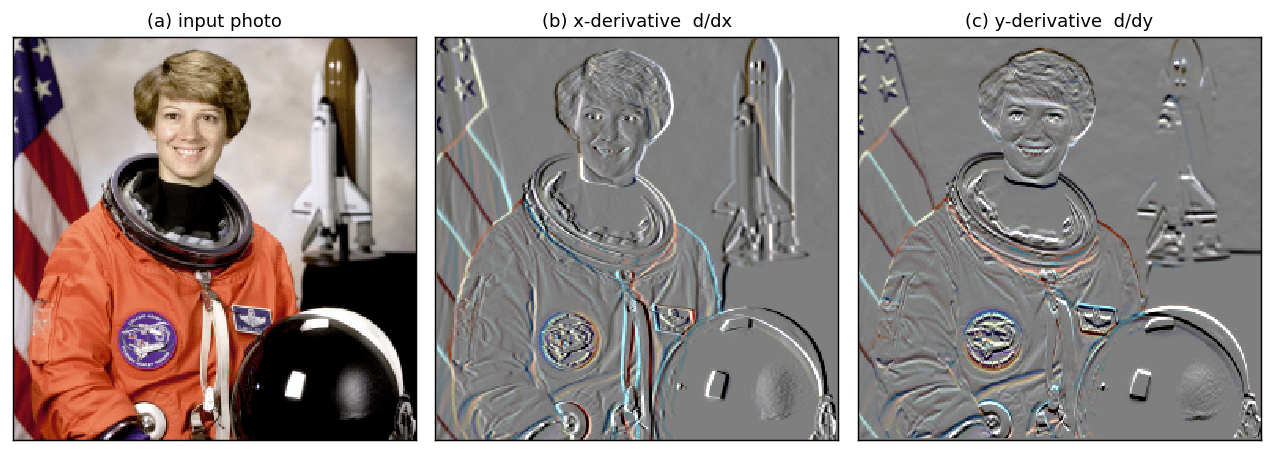

# Figure 18.2: x/y derivatives of a color photo, shown the book's way:
# the SIGNED derivative of each color channel around mid-gray (blue/orange edges).
# stand-in for a color photograph of the MIT dome in the book; original: https://visionbook.mit.edu/figures/derivatives/mit_der_a.jpg
photo = photo_rgb
dx = conv2d_rgb(photo, D1)
dy = conv2d_rgb(photo, D1.T)

print('mean |d/dx|:', dx.abs().mean().item(), ' mean |d/dy|:', dy.abs().mean().item())

mean |d/dx|: 0.03433092311024666  mean |d/dy|: 0.027904972434043884

What the two kernels do in frequency

An ideal derivative multiplies each frequency by

j\omega

, i.e. magnitude grows linearly with frequency. The DFTs

D_0[u] = 1-e^{-2\pi j u/N},\ |D_0| = 2\sin(\pi u/N),\qquad D_1[u] = j\sin(2\pi u/N),

both approximate

|\omega|

at low frequencies.

|D_0|

tracks the ideal further up the band;

|D_1|

rolls off earlier (it suppresses the highest frequencies, so it is smoother and less noisy).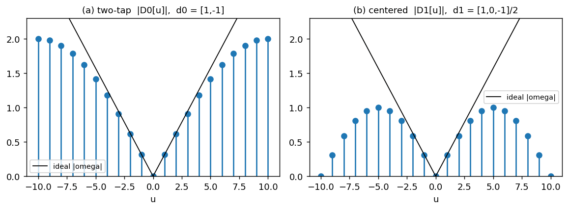

# Figure 18.4: |DFT| of d0 and d1 vs the ideal |omega|, as discrete stems over
# u = -N/2 .. N/2 (as the book draws them), with the ideal shown as a line.
N = 20
u = np.arange(-N // 2, N // 2 + 1)             # -10 .. 10
ideal = np.abs(2 * np.pi * u / N)              # ideal derivative response |omega|
D0m = np.abs(1 - np.exp(-2j * np.pi * u / N))  # = 2 sin(pi u / N)
D1m = np.abs(np.sin(2 * np.pi * u / N))

Gaussian derivatives beat noise

Differentiation amplifies high frequencies, so a raw

[1,-1]

derivative of a noisy image is dominated by noise. Because differentiation and convolution commute,

\frac{\partial \ell}{\partial x}*g = \ell * \frac{\partial g}{\partial x},

you can differentiate the smooth Gaussian instead of the noisy image. The first Gaussian derivative

g_x=-\tfrac{x}{\sigma^2}g

smooths and differentiates in one pass. Figure 18.6 contrasts the two on a noisy photo (the book’s version).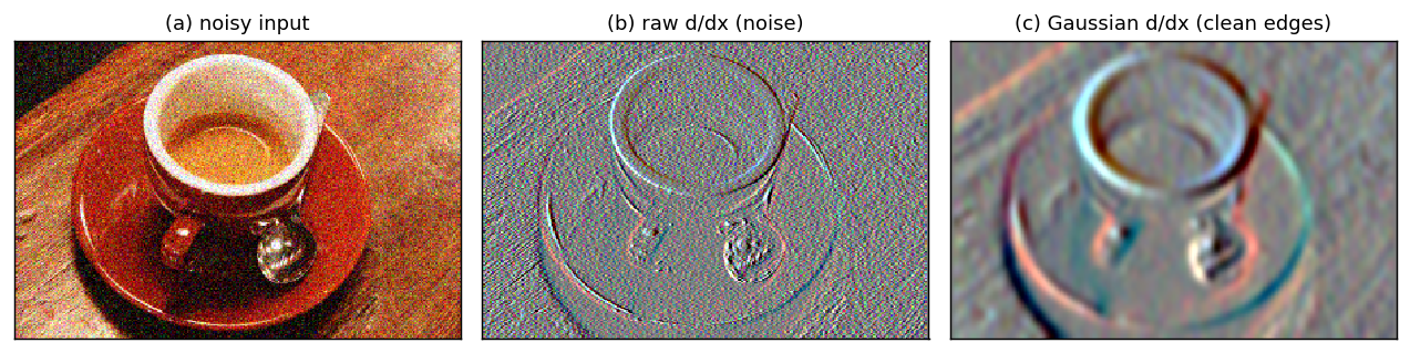

# Figure 18.6: raw x-derivative (noise-amplified) vs Gaussian x-derivative.
# Shown the way the book does it: the SIGNED derivative of each color channel,
# displayed around mid-gray (light = positive edge, dark = negative edge).
# stand-in for a noisy photograph of a stop sign in the book; original: https://visionbook.mit.edu/figures/derivatives/stop_noise.jpg
noisy = (coffee_rgb + 0.12 * torch.randn_like(coffee_rgb)).clamp(0, 1)   # additive Gaussian noise
raw = conv2d_rgb(noisy, D1)                                 # raw centered difference, per channel
gauss = conv2d_rgb(noisy, gauss_deriv2d(3.0, 1, 0))         # Gaussian x-derivative, sigma=3

print('background derivative std, raw   :', raw[:80, :80].std().item())
print('background derivative std, gauss :', gauss[:80, :80].std().item(),
      '  # Gaussian derivative suppresses the noise floor')

background derivative std, raw   : 0.08325188606977463
background derivative std, gauss : 0.008138191886246204   # Gaussian derivative suppresses the noise floor

Gaussian derivatives and the Hermite family

Higher derivative orders of the Gaussian are Hermite polynomials times the Gaussian:

g_{x^n}(x;\sigma) = \Bigl(\tfrac{-1}{\sigma\sqrt2}\Bigr)^n H_n\!\Bigl(\tfrac{x}{\sigma\sqrt2}\Bigr)\,g(x;\sigma),\qquad H_n(x)=2xH_{n-1}-2(n-1)H_{n-2}.

Each order adds one more oscillation. Orders 0 to 3 for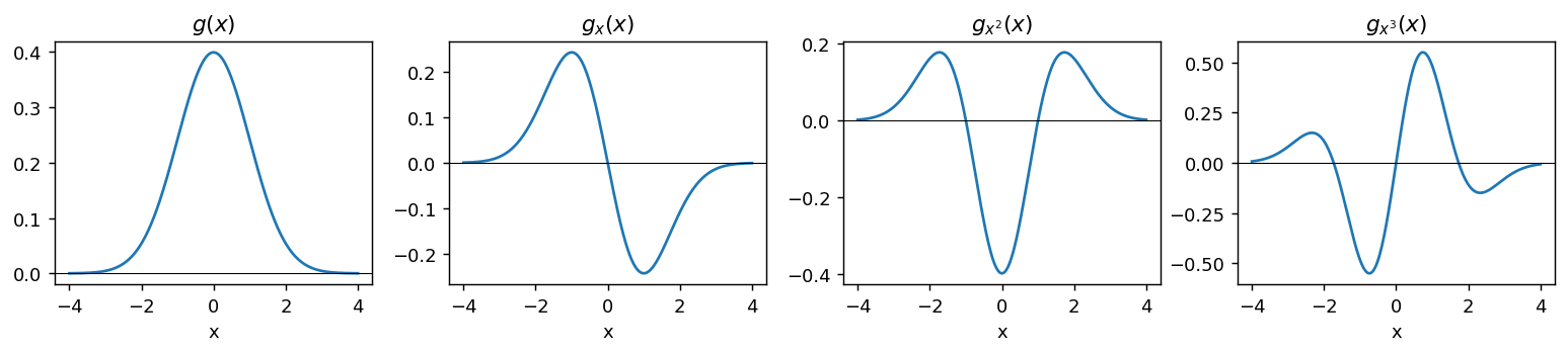

\sigma=1

# Figure 18.9: the Gaussian and its first three derivatives, sigma = 1
# (smooth continuous curves over x in [-4, 4], as in the book).
x = np.linspace(-4, 4, 400)
g = np.exp(-x**2 / 2) / np.sqrt(2 * np.pi)
a = x / np.sqrt(2)
titles = ['$g(x)$', '$g_x(x)$', '$g_{x^2}(x)$', '$g_{x^3}(x)$']

# Sanity: order-0 integrates to ~1 (unit area); every derivative integrates to ~0.
for n in range(4):
    print(f'sum of order {n}:', float(dgauss_1d(1.0, n, radius=8).sum()))

sum of order 0: 1.0
sum of order 1: 0.0
sum of order 2: -2.3798011739017966e-07
sum of order 3: 0.0

The 2-D Gaussian-derivative triangle

Because the 2-D Gaussian is separable, every mixed partial

g_{x^n y^m}

is just the outer product of two 1-D Hermite-weighted Gaussians. Arranged by total order they form a triangle (the top is

g

itself; each row adds one derivative). Each kernel is shown signed around mid-gray. These are exactly the oriented center-surround filters a linear front-end computes.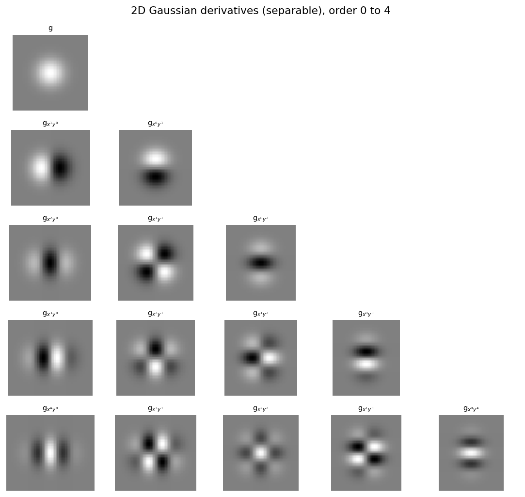

# Figure 18.10: triangle of separable 2D Gaussian derivatives, order 0..4.
K = 4; sig = 6.0

Multiscale Gaussian derivatives

The scale

\sigma

selects which edges survive: small

\sigma

picks up fine texture, large

\sigma

only the coarse structure. Here is the Gaussian x-derivative of a photograph at

\sigma=2,4,8

(the book uses a zebra).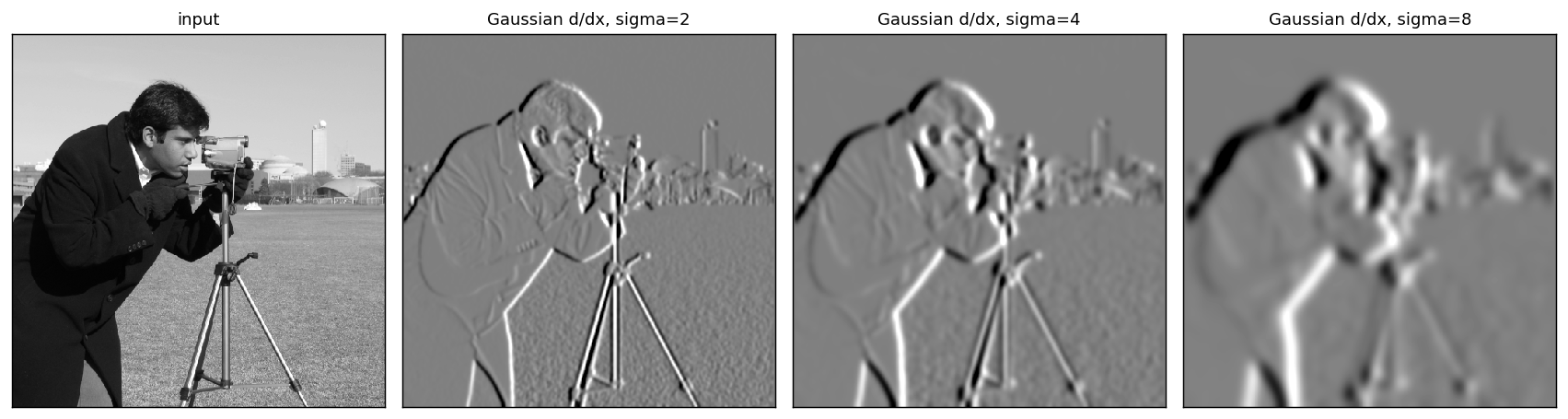

# Figure 18.8: Gaussian x-derivative of a photo at increasing scale,
# shown signed around mid-gray (embossed edges), as in the book.
# stand-in for a photograph of a zebra in the book; original: https://visionbook.mit.edu/derivatives.html#fig-gaussiander_zebra
zebra = camera
panels, titles = [zebra], ['input']
for s in (2.0, 4.0, 8.0):
    resp = conv2d(zebra, gauss_deriv2d(s, 1, 0))
    panels.append(show_signed(resp)); titles.append(f'Gaussian d/dx, sigma={int(s)}')

Derivatives from binomial filters

Convolving a binomial smoother

b_n

(Pascal’s triangle) with the elementary difference

[1,-1]

gives a family of discrete derivative kernels

d_n=b_n*[1,-1]

: smoother as

n

grows, all with DC gain 0.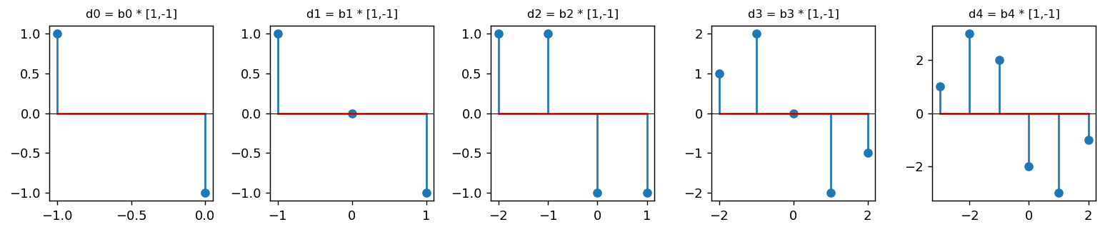

d_0=[1,-1],\quad d_1=[1,0,-1],\quad d_2=[1,1,-1,-1],\quad d_3=[1,2,0,-2,-1],\dots

# The derivative-of-binomial family: d_n = b_n * [1, -1].
def binom(n):
    b = np.array([1.0])
    for _ in range(n):
        b = np.convolve(b, [1.0, 1.0])
    return b

d0: [ 1 -1]  sum = 0
d1: [ 1  0 -1]  sum = 0
d2: [ 1  1 -1 -1]  sum = 0
d3: [ 1  2  0 -2 -1]  sum = 0
d4: [ 1  3  2 -2 -3 -1]  sum = 0

Roberts and Sobel in frequency

The Roberts cross (

2\times2

diagonal differences) and the Sobel-Feldman operator (

[1,0,-1]

derivative

\times

[1,2,1]

smoothing) are the classic 2-D edge operators. Sobel is separable,

\text{Sobel}_x = [1,0,-1]\otimes[1,2,1]^\top

, and its smoothing makes it the most isotropic and noise-tolerant. The 2-D DFT magnitudes below show each operator’s directional selectivity.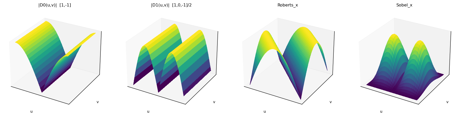

# Figure 18.14: 2D |DFT| SURFACES of d0, d1, Roberts_x, Sobel_x (as in the book).
def dft_mag(kernel, N=64):
    k = np.zeros((N, N)); kh, kw = kernel.shape
    k[:kh, :kw] = kernel                                   # place at origin
    return np.abs(np.fft.fftshift(np.fft.fft2(k)))

kernels = {
    '|D0(u,v)|  [1,-1]': np.array([[1.0, -1.0]]),
    '|D1(u,v)|  [1,0,-1]/2': np.array([[1.0, 0.0, -1.0]]) / 2,
    'Roberts_x': np.array([[1.0, 0.0], [0.0, -1.0]]),
    'Sobel_x': np.array([[1.0, 0.0, -1.0], [2.0, 0.0, -2.0], [1.0, 0.0, -1.0]]),
}
uv = np.linspace(-0.5, 0.5, 64)
U, V = np.meshgrid(uv, uv)

Image gradient and directional derivatives

The gradient

\nabla\ell=(\partial_x\ell,\partial_y\ell)

is a per-pixel vector. The derivative in any direction

\mathbf t=(\cos\theta,\sin\theta)

is just a linear combination of the two you already have, with no new convolution needed:

\frac{\partial\ell}{\partial\mathbf t} = \cos\theta\,\partial_x\ell + \sin\theta\,\partial_y\ell.

# Figure 18.15: directional derivatives of a disc: d/dx, d/dy, d/d45, plus the
# gradient magnitude |grad I| and the gradient ORIENTATION as a color wheel
# (hue = angle), exactly as the book lays it out.
import math
import matplotlib.colors as mcolors
yy, xx = torch.meshgrid(torch.linspace(-1, 1, 256), torch.linspace(-1, 1, 256), indexing='ij')
disc = (xx**2 + yy**2 < 0.5**2).float()
smooth = torch.outer(gaussian_1d(2.0), gaussian_1d(2.0))     # anti-alias the hard edge
disc = conv2d(disc, smooth)
dx = conv2d(disc, D1); dy = conv2d(disc, D1.T)
d45 = math.cos(math.pi / 4) * dx + math.sin(math.pi / 4) * dy
mag = torch.sqrt(dx**2 + dy**2)
ang = torch.atan2(dy, dx)                                    # -pi .. pi
hue = ((ang / (2 * math.pi)) % 1.0).numpy()                  # 0 .. 1
val = (mag / mag.max()).clamp(0, 1).numpy() ** 0.5           # brightness = edge strength
angle_rgb = mcolors.hsv_to_rgb(np.stack([hue, np.ones_like(hue), val], axis=-1))

The Laplacian and Laplacian-of-Gaussian

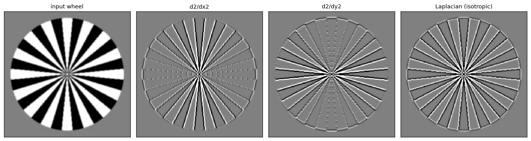
The Laplacian

\nabla^2\ell=\partial_{xx}\ell+\partial_{yy}\ell

is the simplest rotationally invariant second-order operator. Smoothed with a Gaussian it becomes the Laplacian-of-Gaussian (the Mexican-hat wavelet),

\nabla^2 g = \frac{x^2+y^2-2\sigma^2}{\sigma^4}\,g(x,y;\sigma),

a center-surround kernel that responds to blobs and zero-crosses at edges. The book shows the second derivatives on a photograph of a wheel; below, a synthetic spoked wheel has edges at every orientation, which is what tests isotropy.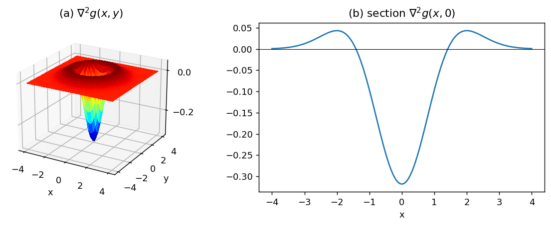

# Figure 18.16: Laplacian-of-Gaussian (Mexican hat), sigma = 1, x,y in [-4, 4].
# Plotted as grad^2 g (NOT negated): a well that dips to ~-0.3 with a positive rim.
xx = np.linspace(-4, 4, 121)
X, Y = np.meshgrid(xx, xx)
sig = 1.0
g = np.exp(-(X**2 + Y**2) / (2 * sig**2)) / (2 * np.pi * sig**2)
log = (X**2 + Y**2 - 2 * sig**2) / sig**4 * g          # grad^2 g

# Figure 18.18: second derivatives of a spoked wheel: d2/dx2, d2/dy2, and their sum
# (the Laplacian) is rotationally invariant. Five-point stencil:
#   [[0,1,0],[1,-4,1],[0,1,0]].
wy, wx = torch.meshgrid(torch.linspace(-1, 1, 256), torch.linspace(-1, 1, 256), indexing='ij')
# stand-in for a photograph of a wheel in the book; original: https://visionbook.mit.edu/figures/spatial_filters/wheel256.jpg
spokes = (torch.cos(16 * torch.atan2(wy, wx)) > 0).float()                  # 16 spokes
wheel = torch.where(wx**2 + wy**2 < 0.9**2, 0.15 + 0.7 * spokes, torch.full_like(wx, 0.5))
wheel = conv2d(wheel, torch.outer(gaussian_1d(1.0), gaussian_1d(1.0)))       # soften aliasing
dxx = conv2d(wheel, torch.tensor([[1.0, -2.0, 1.0]]))          # d2/dx2
dyy = conv2d(wheel, torch.tensor([[1.0], [-2.0], [1.0]]))      # d2/dy2
lap = conv2d(wheel, torch.tensor([[0., 1., 0.], [1., -4., 1.], [0., 1., 0.]]))

print('max |dxx+dyy - Laplacian|:', (dxx + dyy - lap).abs().max().item())

max |dxx+dyy - Laplacian|: 1.1920928955078125e-07

Sharpening: unsharp masking

Subtracting a blurred copy from twice the image boosts the high frequencies the blur removed:

\text{sharpen} = 2\mathbf I - b_{2,2},\qquad \text{DC gain} = 1.

Applied repeatedly it keeps enhancing edges (until artifacts appear). The photo is in color, so the sharpen kernel is applied to each channel independently. The book uses a photograph of a boat.

# Figure 18.23: unsharp masking applied 1..5 times to a color photo.
# stand-in for a photograph of a boat in the book; original: https://visionbook.mit.edu/figures/spatial_filters/boat_sharp0.jpg
boat = coffee_rgb
b = torch.tensor([1.0, 2.0, 1.0]); blur = torch.outer(b, b); blur = blur / blur.sum()
sharpen = torch.zeros(3, 3); sharpen[1, 1] = 2.0; sharpen = sharpen - blur   # 2I - b22

panels, titles = [boat], ['original']
cur = boat
for i in range(1, 6):
    cur = conv2d_rgb(cur, sharpen).clamp(0, 1)
    panels.append(cur); titles.append(f'sharpen x{i}')

print('sharpen kernel DC gain:', float(sharpen.sum()))

sharpen kernel DC gain: 1.0

Retinex: separating reflectance from illumination

An image is reflectance times illumination,

\ell=r\cdot l

. In the log domain this is a sum, and Land’s Retinex exploits a statistical gap: reflectance edges are sharp (large log-gradients) while illumination varies smoothly (small gradients). So you threshold the log-gradient: keep the large part as reflectance, integrate it back with a (mirror-padded) Poisson solve, and take the smooth remainder as illumination. The test setup follows the book: a synthetic Mondrian (piecewise-constant reflectance patches) under a smooth, left-bright illumination, laid out as the book’s

\ell(x,y)=r(x,y)\cdot l(x,y)

decomposition. Because the ground truth is known, you can measure the recovery: the smooth illumination is recovered almost exactly (correlation ~0.97), and the reflectance comes out flat (~0.77; the residual is faint illumination the single global threshold cannot fully separate).

# Figure 18.25/26: Retinex on a synthetic Mondrian x smooth illumination,
# laid out as the book's  l(x,y) = r(x,y) x l(x,y)  decomposition.
def fdx(a): return torch.roll(a, -1, dims=1) - a          # forward difference f[n+1]-f[n]
def fdy(a): return torch.roll(a, -1, dims=0) - a

def poisson_periodic(gx, gy):
    H, W = gx.shape
    fy = np.fft.fftfreq(H)[:, None]; fx = np.fft.fftfreq(W)[None, :]
    Dx = np.exp(2j * np.pi * fx) - 1; Dy = np.exp(2j * np.pi * fy) - 1
    Gx = np.fft.fft2(gx); Gy = np.fft.fft2(gy)
    denom = np.abs(Dx)**2 + np.abs(Dy)**2; denom[0, 0] = 1.0
    Fh = (np.conj(Dx) * Gx + np.conj(Dy) * Gy) / denom; Fh[0, 0] = 0.0
    return np.real(np.fft.ifft2(Fh))

def integrate(gx, gy):
    """Integrate a gradient field. The gradients are MIRROR-reflected first so the
    periodic FFT solve behaves like a Neumann boundary, without this the recovered
    reflectance keeps a low-frequency illumination ramp.
    """
    gx = gx.numpy(); gy = gy.numpy(); H, W = gx.shape
    GX = np.block([[gx, -gx[:, ::-1]], [gx[::-1, :], -gx[::-1, ::-1]]])
    GY = np.block([[gy, gy[:, ::-1]], [-gy[::-1, :], -gy[::-1, ::-1]]])
    f = poisson_periodic(GX, GY)[:H, :W]
    return torch.tensor(f, dtype=torch.float32)

def corr(a, b):
    a = a.flatten() - a.mean(); b = b.flatten() - b.mean()
    return (a * b).sum() / (a.norm() * b.norm() + 1e-12)

# Ground truth: a rich Mondrian (distinct gray levels) under a smooth,
# left-bright illumination, the book's test image.
_ = torch.manual_seed(7)
gyN, gxN, ps = 8, 16, 18
H, Wd = gyN * ps, gxN * ps                          # 144 x 288, wide like the book
levels = torch.tensor([0.18, 0.32, 0.46, 0.60, 0.74, 0.90])
patch = levels[torch.randint(0, len(levels), (gyN, gxN))]
R_true = patch.repeat_interleave(ps, 0).repeat_interleave(ps, 1)
yy, xx = torch.meshgrid(torch.linspace(0, 1, H), torch.linspace(0, 1, Wd), indexing='ij')
L_true = 0.18 + 0.82 * torch.exp(-(((xx - 0.16)**2) / (2 * 0.22**2)
                                    + ((yy - 0.40)**2) / (2 * 0.50**2)))
ell = (R_true * L_true).clamp(1e-3, 1.0)

# Retinex: threshold log-gradients, keep the sharp (reflectance) part, integrate.
logL = torch.log(ell)
gx, gy = fdx(logL), fdy(logL)
T = torch.quantile(torch.stack([gx.abs(), gy.abs()]).flatten(), 0.86)
gxr = torch.where(gx.abs() > T, gx, torch.zeros_like(gx))
gyr = torch.where(gy.abs() > T, gy, torch.zeros_like(gy))
logR = integrate(gxr, gyr); logR = logR - logR.mean() + logL.mean()
R_hat = torch.exp(logR).clamp(0, 2)
L_hat = ell / (R_hat + 1e-3)                        # illumination = smooth remainder

print('corr(recovered reflectance,  truth):', corr(R_hat, R_true).item())
print('corr(recovered illumination, truth):', corr(L_hat, L_true).item())

corr(recovered reflectance,  truth): 0.7698575854301453
corr(recovered illumination, truth): 0.9723199605941772

Concluding remarks

Operator	Kernel	Property
two-tap $d_0$	$[1,-1]$	half-pixel shift, widest band
centered $d_1$	$[1,0,-1]/2$	no shift, smoother
Gaussian deriv	$-\tfrac{x}{\sigma^2}g$	smooths + differentiates; scale-selective
Sobel	$[1,0,-1]\otimes[1,2,1]$	separable, isotropic, noise-tolerant
Laplacian	$[[0,1,0],[1,-4,1],[0,1,0]]$	rotationally invariant, zero-crossings at edges
sharpen	$2\mathbf I - b_{2,2}$	high-boost, DC gain 1

From a single idea, differencing neighboring pixels, the chapter builds edge detection, scale selection (Gaussian derivatives), the isotropic Laplacian, sharpening, and gradient-domain reasoning strong enough to separate reflectance from illumination. These operators are the front end of nearly every classical vision pipeline (SIFT, HOG) and echo the center-surround receptive fields of early biological vision.

Edit this page on GitHub or file an issue.

Perception

Image Processing

CNNs

Scene Understanding

Faster RCNN Lab

YOLO Lab

UNet Lab

Mask RCNN Lab

Measuring Change with Image Derivatives

Discretizing the image derivative

What the two kernels do in frequency

Gaussian derivatives beat noise

Gaussian derivatives and the Hermite family

The 2-D Gaussian-derivative triangle

Multiscale Gaussian derivatives

Derivatives from binomial filters

Roberts and Sobel in frequency

Image gradient and directional derivatives

The Laplacian and Laplacian-of-Gaussian

Sharpening: unsharp masking

Retinex: separating reflectance from illumination

Concluding remarks

​Discretizing the image derivative

​What the two kernels do in frequency

​Gaussian derivatives beat noise

​Gaussian derivatives and the Hermite family

​The 2-D Gaussian-derivative triangle

​Multiscale Gaussian derivatives

​Derivatives from binomial filters

​Roberts and Sobel in frequency

​Image gradient and directional derivatives

​The Laplacian and Laplacian-of-Gaussian

​Sharpening: unsharp masking

​Retinex: separating reflectance from illumination

​Concluding remarks

Discretizing the image derivative

What the two kernels do in frequency

Gaussian derivatives beat noise

Gaussian derivatives and the Hermite family

The 2-D Gaussian-derivative triangle

Multiscale Gaussian derivatives

Derivatives from binomial filters

Roberts and Sobel in frequency

Image gradient and directional derivatives

The Laplacian and Laplacian-of-Gaussian

Sharpening: unsharp masking

Retinex: separating reflectance from illumination

Concluding remarks