This notebook does two things:
  1. Extracts dimensioning-relevant excerpts from the three foundational papers — ResNet (He et al., CVPR 2016), Identity Mappings (He et al., ECCV 2016), and FPN (Lin et al., CVPR 2017).
  2. Demonstrates the preferred, modern featurizer pattern: a ResNet-style backbone with identity shortcuts when shapes match, 1×1 projection shortcuts when they don’t, feeding into an FPN neck that unifies all pyramid levels to d=256d=256 channels.
Papers (arXiv identifiers):
  • ResNet: arXiv:1512.03385
  • Identity mappings: arXiv:1603.05027
  • FPN: arXiv:1612.03144

1) Dimensioning-relevant excerpts (text) and figure takeaways

A. ResNet (He et al., CVPR 2016)

Short excerpt (dimension matching via projection; note the explicit stride-2 handling):
“The projection shortcut … is used to match dimensions (done by 1×1 convolutions).”
(He et al., 2016, Sec. 3.3)
“When the shortcuts go across feature maps of two sizes, they are performed with a stride of 2.”
(He et al., 2016, Sec. 3.3)
(He et al., 2016, Sec. 3.3) Short excerpt (options for increased dimensions):
“(A) … identity mapping, with extra zero entries padded … (B) … projection shortcut … to match dimensions”
(He et al., 2016, Sec. 3.3)
Figure takeaways (do not reproduce the copyrighted figures here; consult the paper figures directly):
  • ResNet Fig. 3 (residual block): illustrates the residual branch F(x)F(x) and the shortcut branch being added; addition requires exact shape match.
  • ResNet Fig. 5 (bottleneck block): shows the 1×1–3×3–1×1 pattern that reduces then restores channels (e.g., 256→64→64→256); the shortcut is typically identity when input/output shapes match.

B. Identity Mappings (He et al., ECCV 2016)

Short excerpt (why identity shortcuts are special in signal propagation):
“forward and backward signals can be directly propagated … when using identity mappings as the skip connections …”
(He et al., 2016, Abstract) (He et al., 2016, Abstract)
Figure takeaway:
  • The paper analyzes variants of residual units and shows that moving toward “cleaner” identity shortcuts improves optimization/propagation (conceptual motivation for using projections only when necessary).

C. FPN (Lin et al., CVPR 2017)

Short excerpt (lateral dimension reduction for addition):
“the corresponding bottom-up map (which undergoes a 1×1 convolutional layer to reduce channel dimensions) [is merged] by element-wise addition.”
(Lin et al., 2017, Sec. 3)
Short excerpt (the canonical d=256d=256 design):
“We set d = 256 … thus all extra convolutional layers have 256-channel outputs.”
(Lin et al., 2017, Sec. 3)
Figure takeaways:
  • FPN Fig. 3 (building block): shows upsample (×2) + 1×1 lateral conv then addition, followed by a 3×3 “smoothing” conv. The addition imposes strict spatial and channel alignment.

2) The core dimensional constraint

Let xRB×Cin×H×Wx \in \mathbb{R}^{B \times C_{in} \times H \times W}. A residual unit computes y=F(x)+S(x),y = F(x) + \mathcal{S}(x), and addition requires identical tensor shapes: F(x),S(x)RB×Cout×H×W.F(x), \mathcal{S}(x) \in \mathbb{R}^{B \times C_{out} \times H' \times W'}. Hence the shortcut must handle two mismatches:
  • channel mismatch: CinCoutC_{in} \neq C_{out}
  • spatial mismatch: (H,W)(H,W)(H,W) \neq (H',W') (typically caused by stride-2 downsampling)

Residual block — shortcut options

Addition requires identical tensor shapes: both the residual branch and the shortcut must produce [B,Cout,H,W][B, C_{out}, H', W'].
import math
import torch
import torch.nn as nn
import torch.nn.functional as F

def shape(x):
    return tuple(x.shape)

def report(name, x):
    print(f"{name}: {shape(x)}")

3) ResNet-style block with correct shortcut dimensioning

We implement a standard BasicBlock with:
  • residual branch: 3×3 conv → BN → ReLU → 3×3 conv → BN
  • shortcut:
    • identity if stride=1 and Cin=CoutC_{in}=C_{out}
    • otherwise a 1×1 conv (projection), with the same stride as the residual branch’s downsampling
class BasicBlock(nn.Module):
    def __init__(self, cin: int, cout: int, stride: int = 1):
        super().__init__()
        self.conv1 = nn.Conv2d(cin, cout, kernel_size=3, stride=stride, padding=1, bias=False)
        self.bn1   = nn.BatchNorm2d(cout)
        self.conv2 = nn.Conv2d(cout, cout, kernel_size=3, stride=1, padding=1, bias=False)
        self.bn2   = nn.BatchNorm2d(cout)
        self.relu  = nn.ReLU(inplace=True)

        if stride != 1 or cin != cout:
            # Projection shortcut: matches channels and spatial size.
            self.shortcut = nn.Sequential(
                nn.Conv2d(cin, cout, kernel_size=1, stride=stride, bias=False),
                nn.BatchNorm2d(cout),
            )
        else:
            self.shortcut = nn.Identity()

    def forward(self, x):
        out = self.relu(self.bn1(self.conv1(x)))
        out = self.bn2(self.conv2(out))
        out = out + self.shortcut(x)
        out = self.relu(out)
        return out

3.1) What goes wrong if you try to add mismatched tensors?

Below we show:
  • a block that downsamples and increases channels (stride=2, 64→128)
  • naive identity shortcut fails (shape mismatch)
  • projection shortcut works
# Dummy input
x = torch.randn(2, 64, 56, 56)

# Residual branch that downsamples and changes channels
residual = nn.Sequential(
    nn.Conv2d(64, 128, 3, stride=2, padding=1, bias=False),
    nn.BatchNorm2d(128),
    nn.ReLU(inplace=True),
    nn.Conv2d(128, 128, 3, stride=1, padding=1, bias=False),
    nn.BatchNorm2d(128),
)

Fx = residual(x)
report("x", x)
report("F(x)", Fx)

print("\nAttempting F(x) + x (naive identity shortcut):")
try:
    _ = Fx + x
except RuntimeError as e:
    print("RuntimeError:", str(e).split("\n")[0])

print("\nUsing a projection shortcut (1×1 conv, stride=2):")
proj = nn.Conv2d(64, 128, 1, stride=2, bias=False)
Sx = proj(x)
report("S(x)", Sx)
y = Fx + Sx
report("F(x)+S(x)", y)
x: (2, 64, 56, 56)
F(x): (2, 128, 28, 28)

Attempting F(x) + x (naive identity shortcut):
RuntimeError: The size of tensor a (28) must match the size of tensor b (56) at non-singleton dimension 3

Using a projection shortcut (1×1 conv, stride=2):
S(x): (2, 128, 28, 28)
F(x)+S(x): (2, 128, 28, 28)

3.2) Option A vs. Option B (ResNet paper terminology)

In the ResNet paper’s discussion:
  • Option A: downsample the shortcut (stride 2) and zero-pad channels to match CoutC_{out}.
  • Option B: downsample and project with 1×1 conv to match dimensions.
For FPN-style backbones, Option B is the preferred practical choice because:
  • the feature hierarchy is consumed downstream (e.g., lateral merges), so having a learned projection at stage transitions is robust,
  • and it matches the canonical ResNet-{50,101,152} “option B” design in the CVPR paper.
Below is a small functional illustration of “Option A-like” padding for the channel mismatch (spatial downsample uses strided slicing for simplicity).
def option_a_shortcut(x, cout: int, stride: int):
    # Spatial downsample: emulate stride-2 shortcut by subsampling.
    if stride == 2:
        x_ds = x[:, :, ::2, ::2]
    elif stride == 1:
        x_ds = x
    else:
        raise ValueError("This demo only supports stride 1 or 2.")
    cin = x_ds.shape[1]
    if cin > cout:
        raise ValueError("Option A padding demo expects cin <= cout.")
    if cin == cout:
        return x_ds
    pad_c = cout - cin
    # Pad channels: (N,C,H,W). We pad on the channel dimension by concatenating zeros.
    zeros = torch.zeros(x_ds.shape[0], pad_c, x_ds.shape[2], x_ds.shape[3], device=x_ds.device, dtype=x_ds.dtype)
    return torch.cat([x_ds, zeros], dim=1)

# Demonstrate option A-like shortcut shape matching
x = torch.randn(2, 64, 56, 56)
Sx_a = option_a_shortcut(x, cout=128, stride=2)
report("Option-A-like S(x)", Sx_a)
Option-A-like S(x): (2, 128, 28, 28)

4) A minimal ResNet-like backbone that exposes {C2, C3, C4, C5}

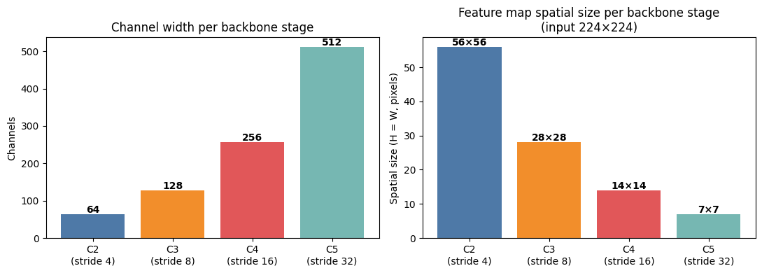
FPN (Lin et al.) uses the outputs of each ResNet stage’s last block: {C2, C3, C4, C5} with strides {4, 8, 16, 32} relative to the input. We build a small backbone that mirrors this structure (conceptually like a tiny ResNet-18).

Backbone stage layout — strides and channel widths

Each stage transition uses a stride-2 first block with a 1×1 projection shortcut (Option B) to match dimensions.
class TinyResNetBackbone(nn.Module):
    def __init__(self):
        super().__init__()
        # Stem (like ResNet): stride-2 conv + stride-2 maxpool => output stride 4
        self.stem = nn.Sequential(
            nn.Conv2d(3, 64, kernel_size=7, stride=2, padding=3, bias=False),
            nn.BatchNorm2d(64),
            nn.ReLU(inplace=True),
            nn.MaxPool2d(kernel_size=3, stride=2, padding=1),
        )
        # Stages: produce C2..C5
        self.layer1 = nn.Sequential(BasicBlock(64,  64, stride=1), BasicBlock(64,  64, stride=1))  # C2, stride 4
        self.layer2 = nn.Sequential(BasicBlock(64, 128, stride=2), BasicBlock(128, 128, stride=1)) # C3, stride 8
        self.layer3 = nn.Sequential(BasicBlock(128,256, stride=2), BasicBlock(256, 256, stride=1)) # C4, stride 16
        self.layer4 = nn.Sequential(BasicBlock(256,512, stride=2), BasicBlock(512, 512, stride=1)) # C5, stride 32

    def forward(self, x):
        x = self.stem(x)
        c2 = self.layer1(x)
        c3 = self.layer2(c2)
        c4 = self.layer3(c3)
        c5 = self.layer4(c4)
        return {"C2": c2, "C3": c3, "C4": c4, "C5": c5}

backbone = TinyResNetBackbone()
x = torch.randn(1, 3, 224, 224)
C = backbone(x)
for k in ["C2","C3","C4","C5"]:
    report(k, C[k])
C2: (1, 64, 56, 56)
C3: (1, 128, 28, 28)
C4: (1, 256, 14, 14)
C5: (1, 512, 7, 7)
import matplotlib.pyplot as plt
import numpy as np

stages = ['C2\n(stride 4)', 'C3\n(stride 8)', 'C4\n(stride 16)', 'C5\n(stride 32)']
channels_bb = [64, 128, 256, 512]
spatial_bb  = [56, 28, 14, 7]

fig, (ax1, ax2) = plt.subplots(1, 2, figsize=(11, 4))
colors = ['#4e79a7', '#f28e2b', '#e15759', '#76b7b2']

bars1 = ax1.bar(stages, channels_bb, color=colors)
ax1.set_ylabel('Channels')
ax1.set_title('Channel width per backbone stage')
for b, v in zip(bars1, channels_bb):
    ax1.text(b.get_x() + b.get_width()/2, b.get_height() + 4, str(v),
             ha='center', fontweight='bold')

bars2 = ax2.bar(stages, spatial_bb, color=colors)
ax2.set_ylabel('Spatial size (H = W, pixels)')
ax2.set_title('Feature map spatial size per backbone stage\n(input 224×224)')
for b, v in zip(bars2, spatial_bb):
    ax2.text(b.get_x() + b.get_width()/2, b.get_height() + 0.4, f'{v}×{v}',
             ha='center', fontweight='bold')

plt.tight_layout()
plt.savefig('backbone_dimensions.png', dpi=120, bbox_inches='tight')
plt.show()
Channel width per backbone stage

5) Preferred FPN module (top-down + lateral, with d=256d=256)

Canonical FPN design choices (as in Lin et al.):
  • 1×1 lateral conv to unify channels to d=256d=256
  • top-down upsample by factor 2 (nearest neighbor is typical)
  • element-wise addition (requires same H×WH \times W and same dd)
  • 3×3 conv “smoothing” on each merged map
  • optional P6P6 via stride-2 3×3 conv on P5P5 (common in detection systems)

FPN top-down pathway — lateral merges and channel unification

The 1×1 lateral convolutions unify heterogeneous backbone channels (64/128/256/512) to a uniform d=256d=256 before the element-wise additions. The additions require strict spatial and channel alignment — which the lateral convolutions and upsample guarantee.
class FPN(nn.Module):
    def __init__(self, c2: int, c3: int, c4: int, c5: int, d: int = 256, make_p6: bool = True):
        super().__init__()
        # Lateral 1×1 convs: Ck -> d
        self.lat2 = nn.Conv2d(c2, d, kernel_size=1)
        self.lat3 = nn.Conv2d(c3, d, kernel_size=1)
        self.lat4 = nn.Conv2d(c4, d, kernel_size=1)
        self.lat5 = nn.Conv2d(c5, d, kernel_size=1)

        # Smoothing 3×3 convs on each pyramid level
        self.smooth2 = nn.Conv2d(d, d, kernel_size=3, padding=1)
        self.smooth3 = nn.Conv2d(d, d, kernel_size=3, padding=1)
        self.smooth4 = nn.Conv2d(d, d, kernel_size=3, padding=1)
        self.smooth5 = nn.Conv2d(d, d, kernel_size=3, padding=1)

        self.make_p6 = make_p6
        self.p6 = nn.Conv2d(d, d, kernel_size=3, stride=2, padding=1) if make_p6 else None

    def forward(self, C):
        c2, c3, c4, c5 = C["C2"], C["C3"], C["C4"], C["C5"]

        m5 = self.lat5(c5)
        m4 = self.lat4(c4) + F.interpolate(m5, scale_factor=2.0, mode="nearest")
        m3 = self.lat3(c3) + F.interpolate(m4, scale_factor=2.0, mode="nearest")
        m2 = self.lat2(c2) + F.interpolate(m3, scale_factor=2.0, mode="nearest")

        p5 = self.smooth5(m5)
        p4 = self.smooth4(m4)
        p3 = self.smooth3(m3)
        p2 = self.smooth2(m2)

        out = {"P2": p2, "P3": p3, "P4": p4, "P5": p5}
        if self.make_p6:
            out["P6"] = self.p6(p5)
        return out

fpn = FPN(c2=64, c3=128, c4=256, c5=512, d=256, make_p6=True)

P = fpn(C)
for k in ["P2","P3","P4","P5","P6"]:
    report(k, P[k])
P2: (1, 256, 56, 56)
P3: (1, 256, 28, 28)
P4: (1, 256, 14, 14)
P5: (1, 256, 7, 7)
P6: (1, 256, 4, 4)

5.1) Sanity checks: the additions are well-defined

Each merge is of the form: M=Lat(C)+Upsample(M+1)M_\ell = \text{Lat}(C_\ell) + \text{Upsample}(M_{\ell+1}) so we assert shape equality at each merge point.
with torch.no_grad():
    c2, c3, c4, c5 = C["C2"], C["C3"], C["C4"], C["C5"]

    m5 = fpn.lat5(c5)
    m4_up = F.interpolate(m5, scale_factor=2.0, mode="nearest")
    m4_lat = fpn.lat4(c4)
    assert m4_up.shape == m4_lat.shape, (m4_up.shape, m4_lat.shape)

    m4 = m4_lat + m4_up
    m3_up = F.interpolate(m4, scale_factor=2.0, mode="nearest")
    m3_lat = fpn.lat3(c3)
    assert m3_up.shape == m3_lat.shape, (m3_up.shape, m3_lat.shape)

    m3 = m3_lat + m3_up
    m2_up = F.interpolate(m3, scale_factor=2.0, mode="nearest")
    m2_lat = fpn.lat2(c2)
    assert m2_up.shape == m2_lat.shape, (m2_up.shape, m2_lat.shape)

print("All FPN merge-shape assertions passed.")
All FPN merge-shape assertions passed.
labels = ['C2/P2\n(stride 4)', 'C3/P3\n(stride 8)', 'C4/P4\n(stride 16)', 'C5/P5\n(stride 32)']
backbone_ch = [64, 128, 256, 512]
fpn_ch      = [256, 256, 256, 256]

x = np.arange(len(labels))
w = 0.35

fig, ax = plt.subplots(figsize=(11, 5))
b1 = ax.bar(x - w/2, backbone_ch, w, label='Backbone Cₖ (heterogeneous)', color='#4e79a7', alpha=0.85)
b2 = ax.bar(x + w/2, fpn_ch,      w, label='FPN output Pₖ (d = 256)',    color='#59a14f', alpha=0.85)

ax.set_ylabel('Number of channels')
ax.set_title('FPN channel unification: heterogeneous backbone → uniform 256-channel pyramid')
ax.set_xticks(x)
ax.set_xticklabels(labels)
ax.legend()
ax.set_ylim(0, 600)
for b, v in [(b1, backbone_ch), (b2, fpn_ch)]:
    for bar, val in zip(b, v):
        ax.text(bar.get_x() + bar.get_width()/2, bar.get_height() + 6,
                str(val), ha='center', fontweight='bold')

plt.tight_layout()
plt.savefig('fpn_channel_unification.png', dpi=120, bbox_inches='tight')
plt.show()
FPN channel unification: heterogeneous backbone to uniform 256-channel pyramid

6) What “preferred approach for FPN” means (operationally)

In a modern featurizer intended for FPN-style consumption, the pragmatic default is:
  1. Backbone (ResNet-style):
    • Identity shortcut if (Cin,H,W)(C_{in}, H, W) matches (Cout,H,W)(C_{out}, H', W')
    • 1×1 projection shortcut (with stride=2 when downsampling) otherwise
      This matches the ResNet paper’s “projection to match dimensions” guidance and the widespread “option B” practice in deep variants.
  2. FPN neck:
    • 1×1 lateral convs to unify all C2..C5C2..C5 to d=256d=256 channels
    • top-down nearest-neighbor upsample by 2
    • elementwise addition
    • 3×3 smoothing conv
    • optional P6P6 from P5P5 via stride-2 3×3 conv
The key theme is the same in both ResNet and FPN: addition enforces strict shape equality, so dimensioning is not a detail—it is the design constraint.

References (primary sources)

  • Kaiming He, Xiangyu Zhang, Shaoqing Ren, Jian Sun. Deep Residual Learning for Image Recognition. CVPR 2016. arXiv:1512.03385.
  • Kaiming He, Xiangyu Zhang, Shaoqing Ren, Jian Sun. Identity Mappings in Deep Residual Networks. ECCV 2016. arXiv:1603.05027.
  • Tsung-Yi Lin, Piotr Dollár, Ross Girshick, Kaiming He, Bharath Hariharan, Serge Belongie. Feature Pyramid Networks for Object Detection. CVPR 2017. arXiv:1612.03144.