

 This section was written by Kaushik Kachireddy (pull request #78), with help from an AI coding agent (Claude Code) on the code. It reproduces the ideas of Chapter 19 of Foundations of Computer Vision by Antonio Torralba, Phillip Isola, and William T. Freeman.
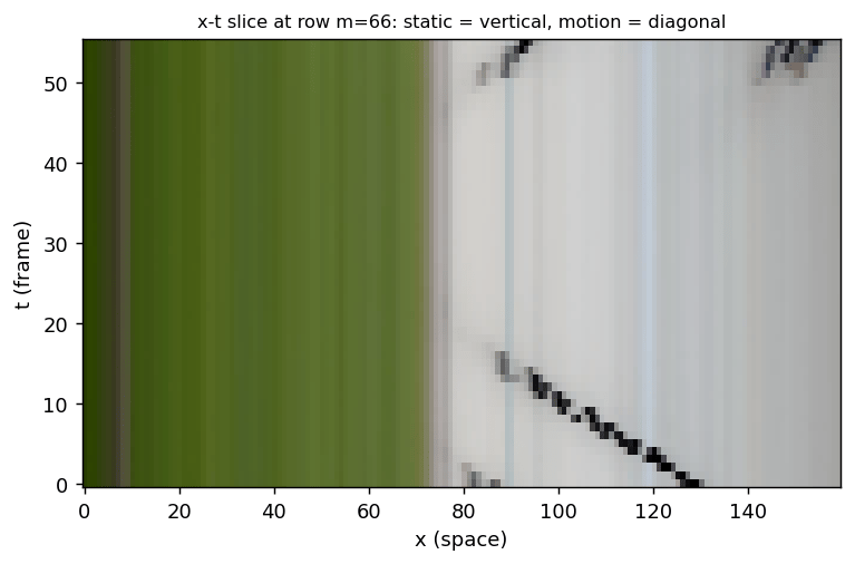
A video is a 3D volume . Once you think of it that way, motion becomes orientation: a static point is a vertical line in the - slice, and a point moving at velocity is a line of slope .
This section builds the chapter’s space-time tools on a real pedestrian video, a static-camera clip of people crossing a plaza (OpenCV’s
This section was written by Kaushik Kachireddy (pull request #78), with help from an AI coding agent (Claude Code) on the code. It reproduces the ideas of Chapter 19 of Foundations of Computer Vision by Antonio Torralba, Phillip Isola, and William T. Freeman.
A video is a 3D volume . Once you think of it that way, motion becomes orientation: a static point is a vertical line in the - slice, and a point moving at velocity is a line of slope .
This section builds the chapter’s space-time tools on a real pedestrian video, a static-camera clip of people crossing a plaza (OpenCV’s vtest.avi sample), the same kind of scene the book uses (Figure 19.1). It covers the - view of motion, its space-time Fourier signature, the spatiotemporal Gaussian and its velocity-skewed form, velocity-tuned blur, spatiotemporal derivatives, and the velocity-nulling filter that erases objects moving at a chosen velocity.
A video is a space-time volume
Stacking the frames along gives a 3-D volume. Slice it at a fixed row and you get an - image: the static background is made of vertical streaks (same for every ), while each walking person traces a diagonal streak whose slope is its velocity. This is the whole idea of the chapter: motion has become orientation.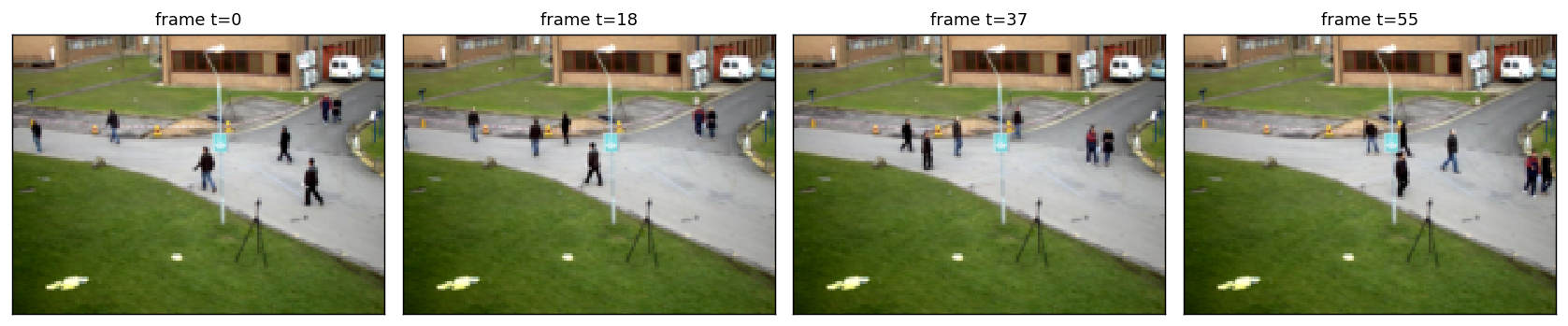
Motion is a slanted plane in the Fourier domain
A globally translating image has all its energy on the plane In 1-D space, a pulse moving at velocity is a slanted band in -, and its 2-D Fourier transform is a sinc ridge lying along the line : vertical for a static pulse, tilting as the speed grows.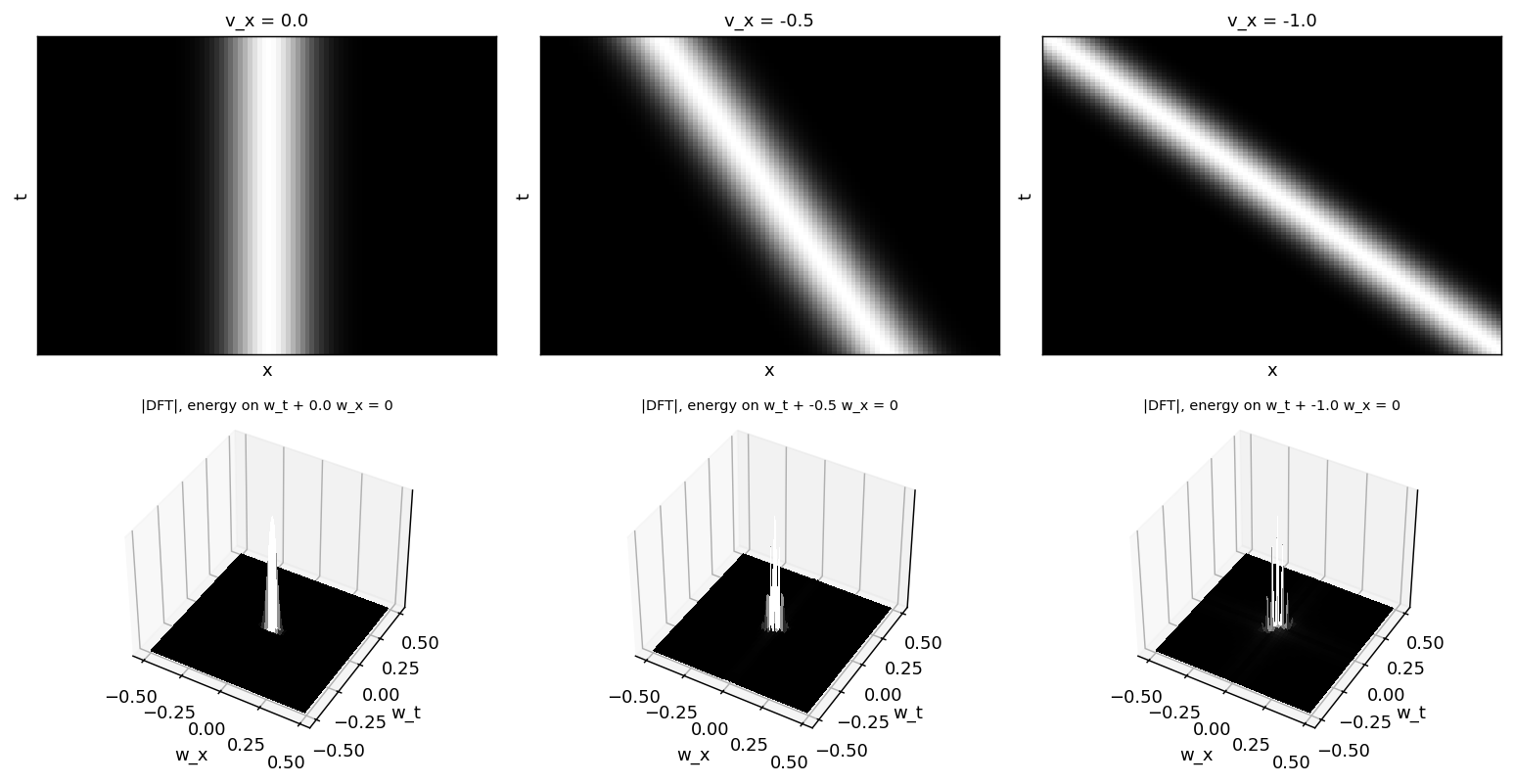
The spatiotemporal Gaussian
The separable space-time Gaussian is an isotropic blob in -. Skewing it along a velocity, , tilts the blob so its long axis follows that motion. Convolving with the skewed kernel is what blurs along a velocity.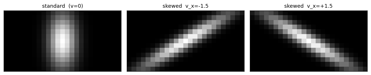
Velocity-tuned (temporal) blur
Averaging the volume along a velocity keeps whatever moves at that velocity sharp (it sits still in the motion-compensated stack) while everything else smears. Tuning to keeps the static background crisp and blurs the walkers; tuning to a walker’s velocity makes that walker snap into focus while the background streaks.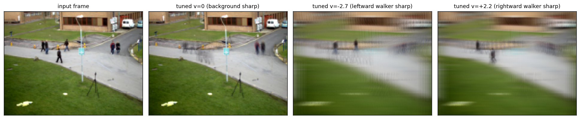
Spatiotemporal Gaussian derivatives
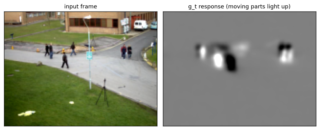
The space-time gradient gives oriented derivative filters. The temporal derivative responds to change over time: it is large exactly where something moves and zero on the static background.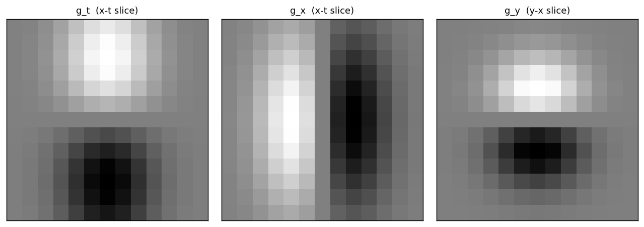
The velocity-nulling filter
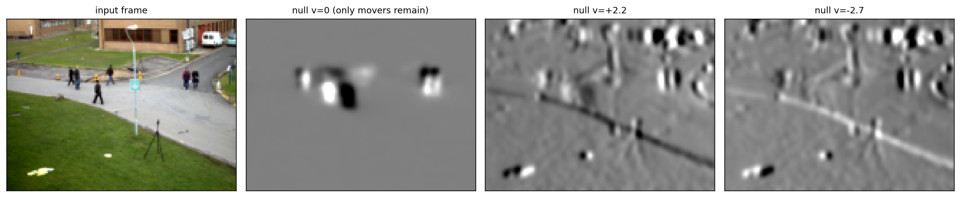
By the brightness-constancy relation, an image moving at exactly satisfies . So the filter annihilates anything moving at while passing everything else. Nulling removes the static background (only the walkers survive); nulling a walker’s velocity erases that walker while the rest remain.
Concluding remarks
Treating time as a third axis turns motion problems into geometry: the same Gaussian, derivative, and steering ideas from the spatial chapters carry over, and the brightness-constancy constraint becomes a single linear filter that can select or reject a velocity. These are the foundations for motion estimation and optical flow.
Found an error on this page? Report an issue.