CNN Example Architectures

This is a very high level view of practical structures of CNNs before the advent of more innovative architectures such as ResNets.

Toy CNN Network

The example CNN architecture above has the following layers:

INPUT [32x32x3] will hold the raw pixel values of the image, in this case an image of width 32, height 32, and with three color channels R,G,B.
CONV layer will compute the output of neurons that are connected to local regions in the input, each computing a dot product between their weights and a small region they are connected to in the input volume. This may result in volume such as [32x32x12] if we decided to use 12 filters.
RELU layer will apply an element-wise ReLU activation function. This leaves the size of the volume unchanged ([32x32x12]).
POOL layer will perform a downsampling operation along the spatial dimensions (width, height), resulting in volume such as [16x16x12].
FC (i.e. fully-connected) layer, also known as a dense layer, will compute the class scores, resulting in volume of size [1x1x10], where each of the 10 numbers correspond to a class score, such as among the 10 categories of the CIFAR-10 dataset that we are showing here.

VGG Networks

The VGG networks from Oxford were the first to use much smaller 3×3 filters in each convolution layer. They have shown that multiple 3×3 convolution in sequence can emulate the effect of larger receptive fields, for examples 5×5 and 7×7. The VGG configuration is shown below:

VGG Configurations: Different columns represent different depths We will focus on configuration D - it was a fairly complex network to train at the time it was authored but its worthy competitor to newer architectures in pure performance terms.

VGG16 Network

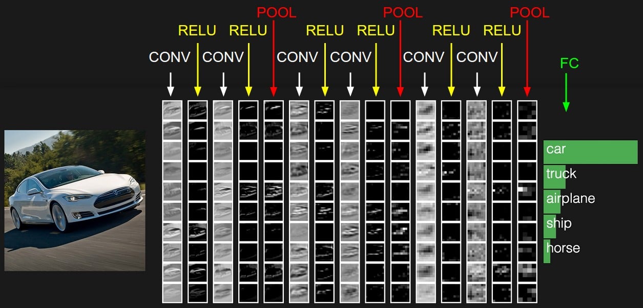
from keras.src import backend
from keras.src import layers
from keras.src.api_export import keras_export
from keras.src.applications import imagenet_utils
from keras.src.models import Functional
from keras.src.ops import operation_utils
from keras.src.utils import file_utils

WEIGHTS_PATH = (
    "https://storage.googleapis.com/tensorflow/keras-applications/"
    "vgg16/vgg16_weights_tf_dim_ordering_tf_kernels.h5"
)
WEIGHTS_PATH_NO_TOP = (
    "https://storage.googleapis.com/tensorflow/"
    "keras-applications/vgg16/"
    "vgg16_weights_tf_dim_ordering_tf_kernels_notop.h5"
)


@keras_export(["keras.applications.vgg16.VGG16", "keras.applications.VGG16"])
def VGG16(
    include_top=True,
    weights="imagenet",
    input_tensor=None,
    input_shape=None,
    pooling=None,
    classes=1000,
    classifier_activation="softmax",
    name="vgg16",
):
    """Instantiates the VGG16 model.

    Reference:
    - [Very Deep Convolutional Networks for Large-Scale Image Recognition](
    https://arxiv.org/abs/1409.1556) (ICLR 2015)

    For image classification use cases, see
    [this page for detailed examples](
      https://keras.io/api/applications/#usage-examples-for-image-classification-models).

    For transfer learning use cases, make sure to read the
    [guide to transfer learning & fine-tuning](
      https://keras.io/guides/transfer_learning/).

    The default input size for this model is 224x224.

    Note: each Keras Application expects a specific kind of input preprocessing.
    For VGG16, call `keras.applications.vgg16.preprocess_input` on your
    inputs before passing them to the model.
    `vgg16.preprocess_input` will convert the input images from RGB to BGR,
    then will zero-center each color channel with respect to the ImageNet
    dataset, without scaling.

    Args:
        include_top: whether to include the 3 fully-connected
            layers at the top of the network.
        weights: one of `None` (random initialization),
            `"imagenet"` (pre-training on ImageNet),
            or the path to the weights file to be loaded.
        input_tensor: optional Keras tensor
            (i.e. output of `layers.Input()`)
            to use as image input for the model.
        input_shape: optional shape tuple, only to be specified
            if `include_top` is `False` (otherwise the input shape
            has to be `(224, 224, 3)`
            (with `channels_last` data format) or
            `(3, 224, 224)` (with `"channels_first"` data format).
            It should have exactly 3 input channels,
            and width and height should be no smaller than 32.
            E.g. `(200, 200, 3)` would be one valid value.
        pooling: Optional pooling mode for feature extraction
            when `include_top` is `False`.
            - `None` means that the output of the model will be
                the 4D tensor output of the
                last convolutional block.
            - `avg` means that global average pooling
                will be applied to the output of the
                last convolutional block, and thus
                the output of the model will be a 2D tensor.
            - `max` means that global max pooling will
                be applied.
        classes: optional number of classes to classify images
            into, only to be specified if `include_top` is `True`, and
            if no `weights` argument is specified.
        classifier_activation: A `str` or callable. The activation function to
            use on the "top" layer. Ignored unless `include_top=True`. Set
            `classifier_activation=None` to return the logits of the "top"
            layer.  When loading pretrained weights, `classifier_activation`
            can only be `None` or `"softmax"`.
        name: The name of the model (string).

    Returns:
        A `Model` instance.
    """
    if not (weights in {"imagenet", None} or file_utils.exists(weights)):
        raise ValueError(
            "The `weights` argument should be either "
            "`None` (random initialization), 'imagenet' "
            "(pre-training on ImageNet), "
            "or the path to the weights file to be loaded.  Received: "
            f"weights={weights}"
        )

    if weights == "imagenet" and include_top and classes != 1000:
        raise ValueError(
            "If using `weights='imagenet'` with `include_top=True`, "
            "`classes` should be 1000.  "
            f"Received classes={classes}"
        )

    # Determine proper input shape
    input_shape = imagenet_utils.obtain_input_shape(
        input_shape,
        default_size=224,
        min_size=32,
        data_format=backend.image_data_format(),
        require_flatten=include_top,
        weights=weights,
    )

    if input_tensor is None:
        img_input = layers.Input(shape=input_shape)
    else:
        if not backend.is_keras_tensor(input_tensor):
            img_input = layers.Input(tensor=input_tensor, shape=input_shape)
        else:
            img_input = input_tensor
    # Block 1
    x = layers.Conv2D(
        64, (3, 3), activation="relu", padding="same", name="block1_conv1"
    )(img_input)
    x = layers.Conv2D(
        64, (3, 3), activation="relu", padding="same", name="block1_conv2"
    )(x)
    x = layers.MaxPooling2D((2, 2), strides=(2, 2), name="block1_pool")(x)

    # Block 2
    x = layers.Conv2D(
        128, (3, 3), activation="relu", padding="same", name="block2_conv1"
    )(x)
    x = layers.Conv2D(
        128, (3, 3), activation="relu", padding="same", name="block2_conv2"
    )(x)
    x = layers.MaxPooling2D((2, 2), strides=(2, 2), name="block2_pool")(x)

    # Block 3
    x = layers.Conv2D(
        256, (3, 3), activation="relu", padding="same", name="block3_conv1"
    )(x)
    x = layers.Conv2D(
        256, (3, 3), activation="relu", padding="same", name="block3_conv2"
    )(x)
    x = layers.Conv2D(
        256, (3, 3), activation="relu", padding="same", name="block3_conv3"
    )(x)
    x = layers.MaxPooling2D((2, 2), strides=(2, 2), name="block3_pool")(x)

    # Block 4
    x = layers.Conv2D(
        512, (3, 3), activation="relu", padding="same", name="block4_conv1"
    )(x)
    x = layers.Conv2D(
        512, (3, 3), activation="relu", padding="same", name="block4_conv2"
    )(x)
    x = layers.Conv2D(
        512, (3, 3), activation="relu", padding="same", name="block4_conv3"
    )(x)
    x = layers.MaxPooling2D((2, 2), strides=(2, 2), name="block4_pool")(x)

    # Block 5
    x = layers.Conv2D(
        512, (3, 3), activation="relu", padding="same", name="block5_conv1"
    )(x)
    x = layers.Conv2D(
        512, (3, 3), activation="relu", padding="same", name="block5_conv2"
    )(x)
    x = layers.Conv2D(
        512, (3, 3), activation="relu", padding="same", name="block5_conv3"
    )(x)
    x = layers.MaxPooling2D((2, 2), strides=(2, 2), name="block5_pool")(x)

    if include_top:
        # Classification block
        x = layers.Flatten(name="flatten")(x)
        x = layers.Dense(4096, activation="relu", name="fc1")(x)
        x = layers.Dense(4096, activation="relu", name="fc2")(x)

        imagenet_utils.validate_activation(classifier_activation, weights)
        x = layers.Dense(
            classes, activation=classifier_activation, name="predictions"
        )(x)
    else:
        if pooling == "avg":
            x = layers.GlobalAveragePooling2D()(x)
        elif pooling == "max":
            x = layers.GlobalMaxPooling2D()(x)

    # Ensure that the model takes into account
    # any potential predecessors of `input_tensor`.
    if input_tensor is not None:
        inputs = operation_utils.get_source_inputs(input_tensor)
    else:
        inputs = img_input

    # Create model.
    model = Functional(inputs, x, name=name)

    # Load weights.
    if weights == "imagenet":
        if include_top:
            weights_path = file_utils.get_file(
                "vgg16_weights_tf_dim_ordering_tf_kernels.h5",
                WEIGHTS_PATH,
                cache_subdir="models",
                file_hash="64373286793e3c8b2b4e3219cbf3544b",
            )
        else:
            weights_path = file_utils.get_file(
                "vgg16_weights_tf_dim_ordering_tf_kernels_notop.h5",
                WEIGHTS_PATH_NO_TOP,
                cache_subdir="models",
                file_hash="6d6bbae143d832006294945121d1f1fc",
            )
        model.load_weights(weights_path)
    elif weights is not None:
        model.load_weights(weights)

    return model


@keras_export("keras.applications.vgg16.preprocess_input")
def preprocess_input(x, data_format=None):
    return imagenet_utils.preprocess_input(
        x, data_format=data_format, mode="caffe"
    )


@keras_export("keras.applications.vgg16.decode_predictions")
def decode_predictions(preds, top=5):
    return imagenet_utils.decode_predictions(preds, top=top)


preprocess_input.__doc__ = imagenet_utils.PREPROCESS_INPUT_DOC.format(
    mode="",
    ret=imagenet_utils.PREPROCESS_INPUT_RET_DOC_CAFFE,
    error=imagenet_utils.PREPROCESS_INPUT_ERROR_DOC,
)
decode_predictions.__doc__ = imagenet_utils.decode_predictions.__doc__

Number of channels

In the VGG-16 model above we can see a common pattern: the number of channels increases as we go deeper into the network. The rationale goes beyond an empirical performance improvement relative to other settings of the number of convolutional filters. The first few layers in the network learn low-level and local features such as edges and corners. As we go deeper into the network, the layers learn more complex features that are compositions of the lower-level features learned in the earlier layers. To effectively capture this growing complexity, the network needs to increase the number of filters or channels to learn more varied and intricate patterns. Another way to describe this is via the effective receptive field of the network that only grows as we go deeper into the network. The deeper layer needs more channels to capture less local patterns that are by definition more complicated.

PyTorch reference

PyTorch class	Description
`nn.Conv2d`	Applies a 2D convolution over an input signal composed of several input planes.
`nn.ReLU`	Applies the rectified linear unit function element-wise.
`nn.MaxPool2d`	Applies a 2D max pooling over an input signal composed of several input planes.
`nn.Flatten`	Flattens a contiguous range of dims into a tensor.
`nn.Linear`	Applies an affine linear transformation to the incoming data: $y = xA^T + b$ .

Key references: (Dumoulin & Visin, 2016; Simonyan & Zisserman, 2014; Peng et al., 2015; Howard et al., 2017; Zeiler & Fergus, 2013)

References

Dumoulin, V., Visin, F. (2016). A guide to convolution arithmetic for deep learning.
Howard, A., Zhu, M., Chen, B., Kalenichenko, D., Wang, W., et al. (2017). MobileNets: Efficient Convolutional Neural Networks for Mobile Vision Applications.
Peng, X., Sun, B., Ali, K., Saenko, K. (2015). What Do Deep CNNs Learn About Objects?.
Simonyan, K., Zisserman, A. (2014). Very Deep Convolutional Networks for Large-Scale Image Recognition.
Zeiler, M., Fergus, R. (2013). Visualizing and Understanding Convolutional Networks.

Edit this page on GitHub or file an issue.

Perception

CNNs

Scene Understanding

Faster RCNN Lab

YOLO Lab

UNet Lab

Mask RCNN Lab

CNN Example Architectures

Toy CNN Network

VGG Networks

Number of channels

PyTorch reference

References

​Toy CNN Network

​VGG Networks

​Number of channels

​PyTorch reference

​References

Toy CNN Network

VGG Networks

Number of channels

PyTorch reference

References