Sampling an Image Without Aliasing

This section was written by Nazib Khan (pull request #46), with help from an AI coding agent on the code. It reproduces the ideas of Chapter 20 of Foundations of Computer Vision by Antonio Torralba, Phillip Isola, and William T. Freeman. The book’s own figures are not reproduced here, because the book’s license covers only the work in full; links point to them instead. This section regenerates the figures of the book’s sampling chapter in PyTorch. Change a parameter in any cell and its figure updates. The thread through the section. Sampling keeps a continuous signal only at instants spaced by

T_s = 1/f_s

. Frequencies separated by a whole multiple of

f_s

then leave identical samples, so the original is no longer recoverable: this is aliasing. The sampling theorem says aliasing is avoided exactly when

f_s > 2 f_{\max}

(the Nyquist rate). Reconstruction fills the gaps between samples, and an anti-aliasing filter band-limits a signal before sampling so the theorem can be honored. Figure 20.15, the cone mosaic of the primate fovea, is a micrograph rather than a computed plot, so a link points to it.

# Every signal in this section is a tensor; a fixed seed keeps the figures reproducible.
import math

import torch
import matplotlib.pyplot as plt
import kornia
from skimage.data import camera

_ = torch.manual_seed(0)
DEVICE = "cuda" if torch.cuda.is_available() else "cpu"

# A dense grid over [0, 1] stands in for the continuous-time axis in the 1-D figures.
t_cont = torch.linspace(0, 1, 2000, device=DEVICE)
print(f"torch {torch.__version__} on {DEVICE} | kornia {kornia.__version__}")

torch 2.11.0+cu130 on cpu | kornia 0.8.3

Images replaced for licensing. The book is published under a CC BY-NC-ND license, which covers only the book as a whole and not its individual images, so this page does not republish the book’s photographs. License-free images stand in for them:

The cameraman photograph (scikit-image) stands in for a photograph of a zebra (Figure 20.16).

If you use the book for non-commercial purposes, you can swap the originals back in: each line that loads a stand-in carries the original’s link in a comment.

Figure 20.1: the continuous wave

The input is a cosine

\ell(t) = \cos(\omega t)

with radian frequency

\omega = 18\pi

, i.e. an ordinary frequency of

\omega/2\pi = 9

Hz, completing nine cycles over the unit interval. This is the signal that sampling has to capture.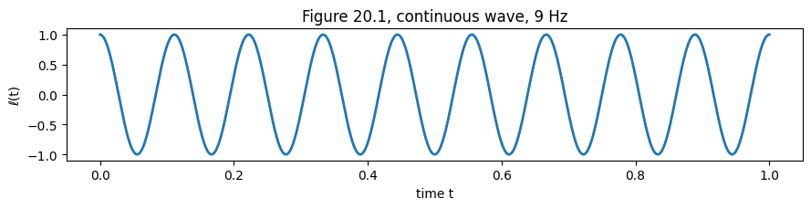

# Continuous input wave: cos(omega t) with omega = 18*pi  ->  9 cycles over [0, 1].
omega = 18 * math.pi                      # radian frequency used by the book
f_in = omega / (2 * math.pi)              # = 9 Hz, the ordinary frequency
wave_in = torch.cos(omega * t_cont)
print(f"input frequency: {f_in:.0f} Hz")

input frequency: 9 Hz

Figure 20.2: sampling the wave

Sample with period

T_s = 1/11

, giving 11 samples across the interval. With 11 samples for 9 periods it seems sufficient, with more samples than periods, yet Nyquist needs

f_s > 18

. The block records the samples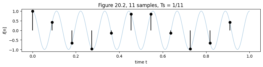

\ell[n] = \ell(n T_s)

# Sample the wave on a coarse grid: period Ts = 1/11  ->  11 instants n*Ts.
fs = 11.0
t_samp = torch.arange(0, 1, 1.0 / fs, device=DEVICE)
samples = torch.cos(omega * t_samp)
print(f"{t_samp.numel()} samples for {f_in:.0f} periods; Nyquist needs fs > {2*f_in:.0f}")

11 samples for 9 periods; Nyquist needs fs > 18

Figure 20.3: many waves, the same samples

Reconstruction is ambiguous: nothing constrains the signal between samples. Under the slow-and-smooth prior the reconstruction is the slowest cosine through the dots. Here the 9 Hz input aliases to

|9 - 11| = 2

Hz: subtracting one sampling rate gives the low frequency that shares every sample, since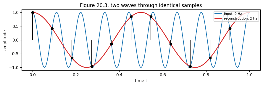

\cos(2\pi\,9\,\tfrac{n}{11}) = \cos(2\pi\,(9-11)\tfrac{n}{11})

# The slow reconstruction: subtract one sampling rate, 9 - 11 = -2 Hz -> 2 Hz.
f_alias = abs(f_in - fs)
wave_recon = torch.cos(2 * math.pi * f_alias * t_cont)

# The 2 Hz reconstruction must match the 9 Hz input at every sample instant.
mismatch = (samples - torch.cos(2 * math.pi * f_alias * t_samp)).abs().max().item()
print(f"reconstruction {f_alias:.0f} Hz vs input {f_in:.0f} Hz: max |mismatch| = {mismatch:.1e}")

reconstruction 2 Hz vs input 9 Hz: max |mismatch| = 3.3e-06

Figure 20.4: aliasing bends a 2-D pattern

The 2-D analogue is

\ell(x,y) = \cos\!\big(2\pi\,a\,(x+y)^2\big)

: diagonal waves whose frequency rises with

(x+y)^2

, slow at the bottom-left and ever finer toward the top-right. Point-sampling to

52\times52

with no pre-filter folds the unrepresentable high frequencies back, and the dominant orientation of the stripes flips.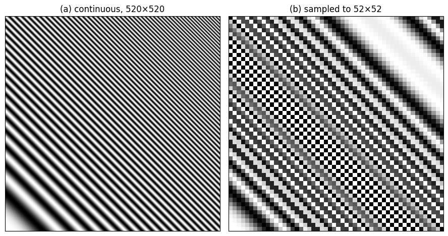

# Diagonal chirp: frequency grows with (x+y), so crests run diagonally and tighten.
N = 520
coords = torch.linspace(0, 1, N, device=DEVICE)
yy, xx = torch.meshgrid(coords, coords, indexing="ij")
pattern = torch.cos(2 * math.pi * 16 * (xx + yy) ** 2)

# Point-sample with no anti-alias pre-filter: keep every stride-th pixel, 520 -> 52.
stride = 10
aliased = pattern[::stride, ::stride]
print(f"continuous {tuple(pattern.shape)} -> point-sampled {tuple(aliased.shape)}")

continuous (520, 520) -> point-sampled (52, 52)

Figure 20.5: a band-limited signal

The sampling theorem is stated for band-limited signals: those whose Fourier transform

L(\omega)

is zero above some maximum frequency

\omega_{\max}

. The sketch below shows such a spectrum, nonzero only inside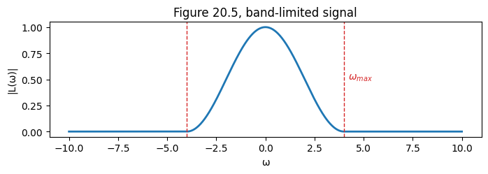

[-\omega_{\max}, \omega_{\max}]

# A schematic band-limited spectrum |L(w)|: a smooth bump confined to |w| < w_max.
w = torch.linspace(-10, 10, 1000, device=DEVICE)
w_max = 4.0
spectrum = torch.where(w.abs() < w_max, torch.cos(math.pi * w / (2 * w_max)) ** 2,
                       torch.zeros_like(w))
print(f"spectrum support: |w| < w_max = {w_max}")

spectrum support: |w| < w_max = 4.0

Figure 20.6: the delta train

Sampling is modelled by multiplying the signal with a delta train (Dirac comb)

\mathrm{III}(t) = \sum_n \delta(t - n T_s)

: impulses at every multiple of

T_s

. Here

T_s = 1

. Arrow heads mark the impulses (each of infinite height, unit area).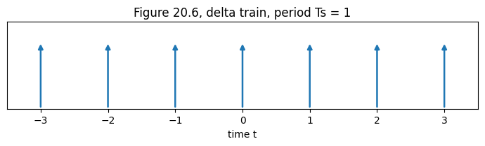

# Delta train with period Ts = 1: impulse locations over a few periods.
Ts_comb = 1.0
impulse_times = torch.arange(-3, 4, Ts_comb)
print(f"impulses at t = {impulse_times.tolist()}")

impulses at t = [-3.0, -2.0, -1.0, 0.0, 1.0, 2.0, 3.0]

Figure 20.7: sampling with the delta train

Multiplying a continuous signal by the delta train keeps its values only at the impulse times, producing the sampled signal

\ell_s(t) = \ell(t)\,\mathrm{III}(t)

. Left: the continuous signal. Right: its delta-sampled version, impulses scaled by the signal.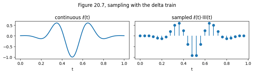

# A smooth low-frequency signal and its delta-train samples.
sig = torch.exp(-((t_cont - 0.5) ** 2) / 0.05) * torch.cos(2 * math.pi * 3 * t_cont)
Ts7 = 0.04
t7 = torch.arange(0, 1, Ts7, device=DEVICE)
sig7 = torch.exp(-((t7 - 0.5) ** 2) / 0.05) * torch.cos(2 * math.pi * 3 * t7)
print(f"continuous samples: {sig.numel()},  delta-train samples: {sig7.numel()}")

continuous samples: 2000,  delta-train samples: 25

Figure 20.8: aliasing in the Fourier domain

Sampling replicates the spectrum: the transform of the sampled signal is

\sum_k L(\omega - k\,\omega_s)

, copies of

L

spaced by the sampling frequency

\omega_s

. (a) When

\omega_s > 2\omega_{\max}

the copies stay separate and the original is recoverable. (b) When

\omega_s < 2\omega_{\max}

neighboring copies overlap; high frequencies leak into low ones. That is aliasing.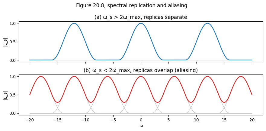

# Replicate the band-limited bump at multiples of the sampling frequency w_s.
def replicate(w_axis, w_s, w_max, n=6):
    total = torch.zeros_like(w_axis)
    copies = []
    for k in range(-n, n + 1):
        shifted = w_axis - k * w_s
        copy = torch.where(shifted.abs() < w_max,
                           torch.cos(math.pi * shifted / (2 * w_max)) ** 2,
                           torch.zeros_like(w_axis))
        copies.append(copy); total = total + copy
    return total, copies

w_axis = torch.linspace(-20, 20, 2000, device=DEVICE)
sep, sep_copies = replicate(w_axis, w_s=12.0, w_max=4.0)   # w_s > 2 w_max -> no overlap
ovl, ovl_copies = replicate(w_axis, w_s=6.0, w_max=4.0)    # w_s < 2 w_max -> overlap
print("case (a) w_s=12 > 8 : no overlap | case (b) w_s=6 < 8 : overlap")

case (a) w_s=12 > 8 : no overlap | case (b) w_s=6 < 8 : overlap

Figure 20.9: the sinc function

Ideal reconstruction convolves the samples with a

\mathrm{sinc}

, the impulse response of the ideal low-pass (box) filter.

\mathrm{sinc}(t) = \sin(\pi t)/(\pi t)

peaks at the origin, is symmetric, and decays as

1/t

with zero crossings at the integers.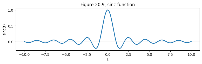

# torch.sinc is the normalized sinc: sin(pi t)/(pi t), zero crossings at integers.
ts = torch.linspace(-10, 10, 2000, device=DEVICE)
sinc = torch.sinc(ts)
print(f"sinc(0) = {torch.sinc(torch.zeros(1)).item():.0f}, zero crossings at integers")

sinc(0) = 1, zero crossings at integers

Figure 20.10: sinc interpolation

The ideal reconstruction is

\hat\ell(t) = \sum_n \ell[n]\,\mathrm{sinc}\!\big((t - nT_s)/T_s\big)

: a scaled, shifted sinc centered on each sample. The thin curves are the individual sincs; their sum (thick) is the smooth interpolation. Each sinc’s zero crossings fall on the other sample locations, so every sample is honoured exactly.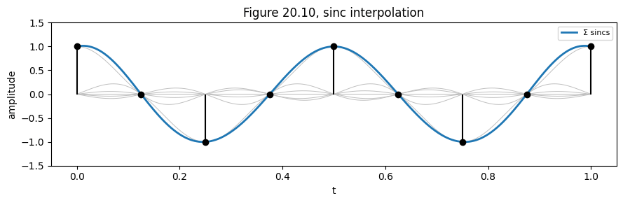

# Reconstruct a slow signal from its samples by summing shifted, scaled sincs.
Ts10 = 1.0 / 8
t10 = torch.arange(0, 1 + Ts10, Ts10, device=DEVICE)
x10 = torch.cos(2 * math.pi * 2 * t10)                       # samples of a 2 Hz wave
# Each sample contributes x[n]*sinc((t - n*Ts)/Ts); stack then sum over samples.
basis = x10[:, None] * torch.sinc((t_cont[None, :] - t10[:, None]) / Ts10)
recon10 = basis.sum(0)
print(f"{t10.numel()} samples reconstructed onto {t_cont.numel()} dense points")

9 samples reconstructed onto 2000 dense points

Figure 20.11: reconstruction degrades with sampling rate

One band-limited signal (a sum of a 3 Hz and 7 Hz cosine, so

f_{\max}=7

) is sampled at three rates. Left: the samples on the signal. Middle: the magnitude spectrum of the samples: peaks land at the true frequencies only while Nyquist holds, otherwise they fold. Right: sinc reconstruction (red) vs the original. Above Nyquist (

f_s>14

) it is exact; below, it is wrong.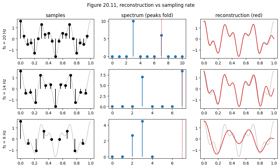

# Band-limited test signal x(t) = cos(2 pi 3 t) + 0.6 cos(2 pi 7 t),  f_max = 7 Hz.
def x_of(t):
    return torch.cos(2 * math.pi * 3 * t) + 0.6 * torch.cos(2 * math.pi * 7 * t)

x_dense = x_of(t_cont)
rates = [20.0, 14.0, 9.0]            # above Nyquist, at Nyquist, below (aliased)
recons, specs, sample_sets = [], [], []
for fr in rates:
    tn = torch.arange(0, 1, 1.0 / fr, device=DEVICE)
    xn = x_of(tn)
    # sinc reconstruction from these samples onto the dense grid
    r = (xn[:, None] * torch.sinc((t_cont[None, :] - tn[:, None]) * fr)).sum(0)
    # magnitude spectrum of the sample sequence
    mag = torch.fft.rfft(xn).abs()
    freqs = torch.fft.rfftfreq(xn.numel(), d=1.0 / fr)
    recons.append(r); specs.append((freqs, mag)); sample_sets.append((tn, xn))
print(f"sampled at rates {rates} Hz (Nyquist = {2*7} Hz)")

sampled at rates [20.0, 14.0, 9.0] Hz (Nyquist = 14 Hz)

Figure 20.12: local interpolation kernels

Ideal sinc reconstruction needs every sample. Cheaper local kernels trade accuracy for support. Nearest interpolation convolves the samples with a box of width

T_s

; linear interpolation convolves with a triangle of width

2T_s

(the convolution of two boxes). Both are shown as the kernel that the samples are convolved with.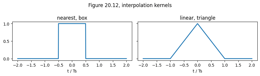

# Nearest = box of width Ts; linear = triangle of width 2 Ts.
tk = torch.linspace(-2, 2, 1000, device=DEVICE)
box = torch.where(tk.abs() <= 0.5, torch.ones_like(tk), torch.zeros_like(tk))
triangle = torch.clamp(1 - tk.abs(), min=0.0)
print("nearest -> box kernel (width Ts) | linear -> triangle kernel (width 2 Ts)")

nearest -> box kernel (width Ts) | linear -> triangle kernel (width 2 Ts)

Figure 20.13: 2-D sampling patterns

Images need not be sampled on a square grid. Three arrangements: a rectangular grid, a hexagonal grid (alternate rows offset by half a step, rows spaced by

\sqrt{3}/2

), and an irregular grid (jittered positions).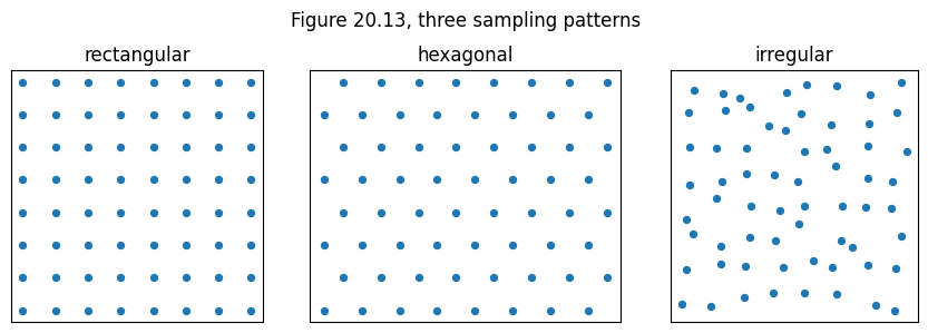

# Build rectangular, hexagonal, and irregular (jittered) sample positions.
n = 8
gx, gy = torch.meshgrid(torch.arange(n), torch.arange(n), indexing="ij")
rect = torch.stack([gx.flatten().float(), gy.flatten().float()], dim=1)

hex_pts = rect.clone()
hex_pts[:, 0] = hex_pts[:, 0] + 0.5 * (hex_pts[:, 1] % 2)     # offset odd rows
hex_pts[:, 1] = hex_pts[:, 1] * (math.sqrt(3) / 2)            # compress row spacing

irate = rect + 0.18 * torch.randn_like(rect)                 # jittered grid
print(f"{rect.shape[0]} points per pattern")

64 points per pattern

Figure 20.14: Fourier transforms of the sampling lattices

In the frequency domain each sampling lattice repeats the spectrum on the reciprocal lattice, and the no-aliasing region is its Voronoi cell (red). The rectangular lattice gives a square cell; the hexagonal lattice gives a hexagon, which packs the largest alias-free area per sample, about a 14% resolution gain.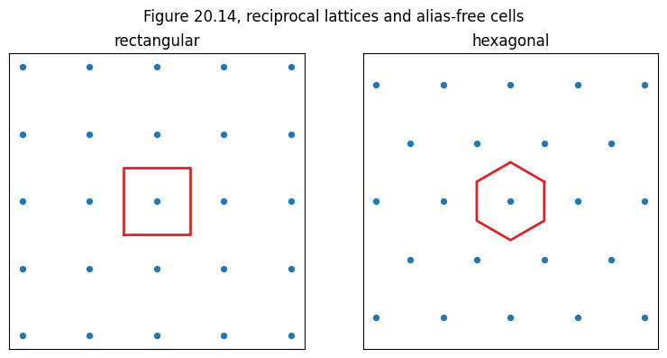

# Reciprocal lattices and their Voronoi cells (the alias-free frequency region).
k = torch.arange(-2, 3)
ax_, ay_ = torch.meshgrid(k, k, indexing="ij")
rect_recip = torch.stack([ax_.flatten().float(), ay_.flatten().float()], dim=1)

hex_recip = rect_recip.clone()                                # reciprocal of a hex lattice
hex_recip[:, 0] = hex_recip[:, 0] + 0.5 * (hex_recip[:, 1] % 2)
hex_recip[:, 1] = hex_recip[:, 1] * (math.sqrt(3) / 2)

square_cell = torch.tensor([[-.5, -.5], [.5, -.5], [.5, .5], [-.5, .5], [-.5, -.5]])
ang = torch.linspace(0, 2 * math.pi, 7)                       # hexagon Voronoi cell
hexa = torch.stack([0.58 * torch.cos(ang + math.pi / 6), 0.58 * torch.sin(ang + math.pi / 6)], 1)
print("rect cell: square | hex cell: hexagon (larger alias-free area)")

rect cell: square | hex cell: hexagon (larger alias-free area)

Figure 20.15: the cone mosaic

The book illustrates that the photoreceptors in the primate fovea sit on an approximately hexagonal lattice, using a micrograph of a monkey retina from Curcio et al. (Figure 20.15). That is measured microscopy, not a computed plot, so there is nothing to regenerate here. The previous figure already shows why hexagonal sampling is favored.

Figure 20.16: aliasing in a real image

The book downsamples a photograph of a zebra and the stripes change orientation. Here the public-domain cameraman test image stands in for it: you point-sample it with no pre-filter at two rates. Reconstructed to full size, the fine detail (tripod, coat texture) breaks up, and the log magnitude spectrum shows energy folding inward.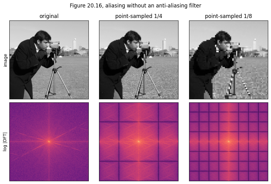

# Load the cameraman test image as a single-channel float tensor in [0, 1].
# stand-in for a photograph of a zebra in the book; original: https://visionbook.mit.edu/sampling_and_aliasing.html#fig-aliasingFTzebra
img = (torch.from_numpy(camera().copy()).float() / 255.0).to(DEVICE)

def point_sample(x, s):
    # keep every s-th pixel (no pre-filter), then nearest-upscale to full size for comparison
    ds = x[::s, ::s]
    return ds.repeat_interleave(s, 0).repeat_interleave(s, 1)[: x.shape[0], : x.shape[1]]

def log_spectrum(x):
    return torch.fft.fftshift(torch.fft.fft2(x)).abs().add(1e-3).log()

aliased_4 = point_sample(img, 4)
aliased_8 = point_sample(img, 8)
print(f"image {tuple(img.shape)} point-sampled at 1/4 and 1/8")

image (512, 512) point-sampled at 1/4 and 1/8

Figure 20.17: the anti-aliasing filter

Blurring with a low-pass filter before sampling removes the frequencies the grid cannot represent, so they no longer fold. The next cell applies a Kornia Gaussian blur, then point-samples at the same 1/8 rate. The result keeps the recognizable low-frequency structure, and its spectrum no longer shows the aliased fold-in, at the cost of the lost (genuinely unrepresentable) detail.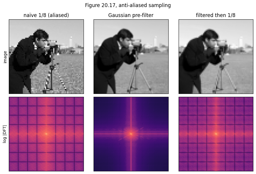

# Anti-alias: Gaussian low-pass (Kornia) BEFORE point-sampling, vs the naive 1/8 above.
def blur(x, ksize, sigma):
    out = kornia.filters.gaussian_blur2d(x[None, None], (ksize, ksize), (sigma, sigma))
    return out[0, 0]

prefiltered = blur(img, 11, 4.0)
antialiased_8 = point_sample(prefiltered, 8)
print("Gaussian pre-filter (sigma=4) applied before 1/8 sampling")

Gaussian pre-filter (sigma=4) applied before 1/8 sampling

Concluding remarks

Aliasing appears whenever a continuous light field is sampled, and again at every downsampling or upsampling step (chapter 21 of the book). The sampling theorem says it is avoided when

f_s > 2 f_{\max}

; when it cannot be (a finite-resolution grid is never band-limited), an anti-aliasing filter trades unrepresentable detail for an artifact-free image. Aliasing is not always harmful: super-resolution methods exploit it to recover detail across frames. Reference. A. Torralba, P. Isola, W. T. Freeman, Foundations of Computer Vision, MIT Press, chapter 20, visionbook.mit.edu.

Edit this page on GitHub or file an issue.

Perception

Image Processing

CNNs

Scene Understanding

Faster RCNN Lab

YOLO Lab

UNet Lab

Mask RCNN Lab

Sampling an Image Without Aliasing

Figure 20.1: the continuous wave

Figure 20.2: sampling the wave

Figure 20.3: many waves, the same samples

Figure 20.4: aliasing bends a 2-D pattern

Figure 20.5: a band-limited signal

Figure 20.6: the delta train

Figure 20.7: sampling with the delta train

Figure 20.8: aliasing in the Fourier domain

Figure 20.9: the sinc function

Figure 20.10: sinc interpolation

Figure 20.11: reconstruction degrades with sampling rate

Figure 20.12: local interpolation kernels

Figure 20.13: 2-D sampling patterns

Figure 20.14: Fourier transforms of the sampling lattices

Figure 20.15: the cone mosaic

Figure 20.16: aliasing in a real image

Figure 20.17: the anti-aliasing filter

Concluding remarks

​Figure 20.1: the continuous wave

​Figure 20.2: sampling the wave

​Figure 20.3: many waves, the same samples

​Figure 20.4: aliasing bends a 2-D pattern

​Figure 20.5: a band-limited signal

​Figure 20.6: the delta train

​Figure 20.7: sampling with the delta train

​Figure 20.8: aliasing in the Fourier domain

​Figure 20.9: the sinc function

​Figure 20.10: sinc interpolation

​Figure 20.11: reconstruction degrades with sampling rate

​Figure 20.12: local interpolation kernels

​Figure 20.13: 2-D sampling patterns

​Figure 20.14: Fourier transforms of the sampling lattices

​Figure 20.15: the cone mosaic

​Figure 20.16: aliasing in a real image

​Figure 20.17: the anti-aliasing filter

​Concluding remarks

Figure 20.1: the continuous wave

Figure 20.2: sampling the wave

Figure 20.3: many waves, the same samples

Figure 20.4: aliasing bends a 2-D pattern

Figure 20.5: a band-limited signal

Figure 20.6: the delta train

Figure 20.7: sampling with the delta train

Figure 20.8: aliasing in the Fourier domain

Figure 20.9: the sinc function

Figure 20.10: sinc interpolation

Figure 20.11: reconstruction degrades with sampling rate

Figure 20.12: local interpolation kernels

Figure 20.13: 2-D sampling patterns

Figure 20.14: Fourier transforms of the sampling lattices

Figure 20.15: the cone mosaic

Figure 20.16: aliasing in a real image

Figure 20.17: the anti-aliasing filter

Concluding remarks