

 This section was written by Kimberly Milner (pull request #51), with help from an AI coding agent on the code. It reproduces the ideas of Chapter 15 of Foundations of Computer Vision by Antonio Torralba, Phillip Isola, and William T. Freeman. The book’s own figures are not reproduced here, because the book’s license covers only the work in full; links point to them instead.
Image filtering is the workhorse of low-level vision: blurring, sharpening, edge detection, and template matching are all the same operation, the convolution of an image with a small kernel. This section regenerates the figures in PyTorch and Kornia, building from continuous and discrete signals, through linear translation-invariant (LTI) systems and convolution, to cross-correlation and template matching.
The thread through the section. A system maps an input signal to an output. The systems worth studying are linear and translation-invariant, and every LTI system is completely described by a single impulse response , applied everywhere by convolution: . Cross-correlation is the same computation without flipping the kernel, which is what template matching uses.
Where the book shows a photograph or a hand sketch, a link points to it, and the filtering operations run on scikit-image test images instead.
This section was written by Kimberly Milner (pull request #51), with help from an AI coding agent on the code. It reproduces the ideas of Chapter 15 of Foundations of Computer Vision by Antonio Torralba, Phillip Isola, and William T. Freeman. The book’s own figures are not reproduced here, because the book’s license covers only the work in full; links point to them instead.
Image filtering is the workhorse of low-level vision: blurring, sharpening, edge detection, and template matching are all the same operation, the convolution of an image with a small kernel. This section regenerates the figures in PyTorch and Kornia, building from continuous and discrete signals, through linear translation-invariant (LTI) systems and convolution, to cross-correlation and template matching.
The thread through the section. A system maps an input signal to an output. The systems worth studying are linear and translation-invariant, and every LTI system is completely described by a single impulse response , applied everywhere by convolution: . Cross-correlation is the same computation without flipping the kernel, which is what template matching uses.
Where the book shows a photograph or a hand sketch, a link points to it, and the filtering operations run on scikit-image test images instead.
Images replaced for licensing. The book is published under a CC BY-NC-ND license, which covers only the book as a whole and not its individual images, so this page does not republish the book’s photographs. License-free images stand in for them:
- The coffee photograph (scikit-image) stands in for a photograph of birds in flight (Figure 15.5).
- The astronaut photograph (scikit-image) stands in for a photograph of a zebra (Figure 15.10).
Signals and images
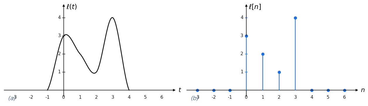
A one-dimensional continuous signal is defined for every real ; sampling it on an integer grid gives the discrete signal . Images are just 2-D discrete signals . Figure 15.1: a continuous signal and its discrete samples.Book Figure 15.1: computed here.
Systems
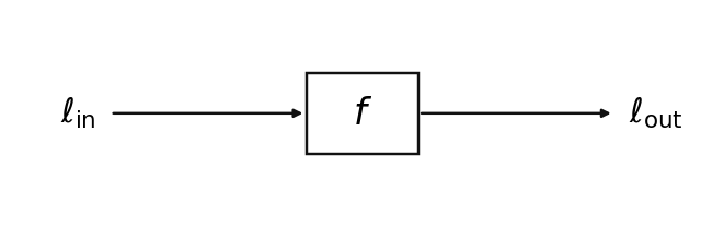
A system maps an input signal to an output signal. The systems that matter here are linear (they respect scaling and superposition) and translation-invariant (shifting the input just shifts the output). Figure 15.2: a system maps an input signal to an output.Book Figure 15.2: drawn as a schematic.
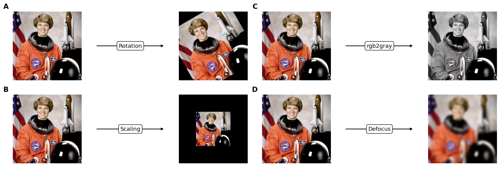
Book Figure 15.3: applied with Kornia.
Convolution
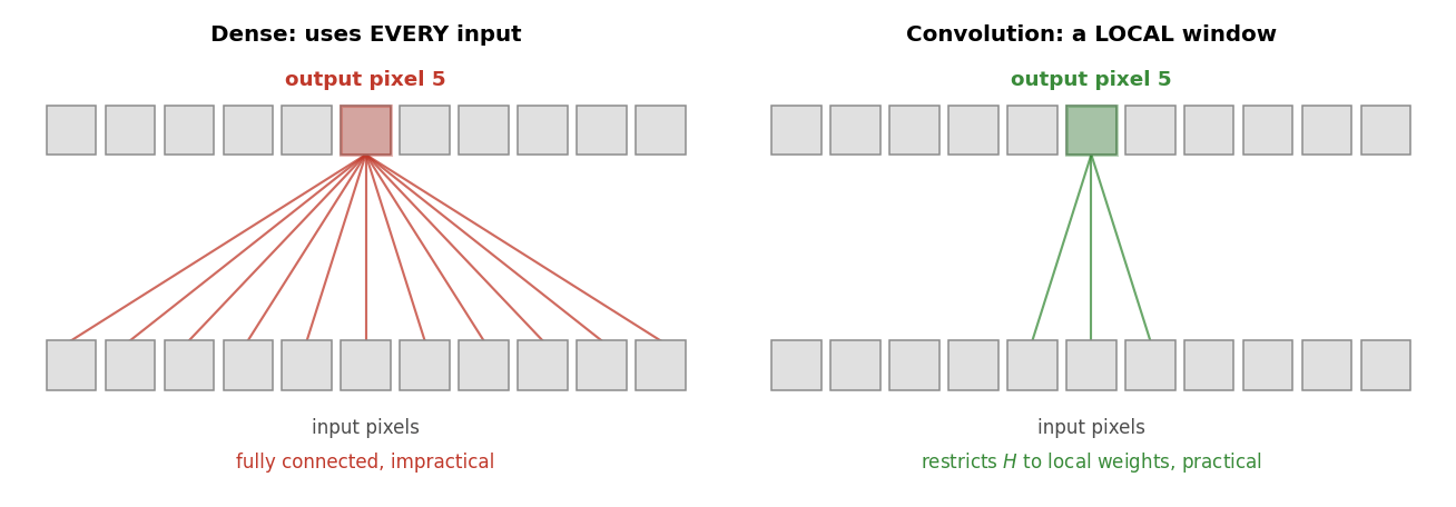
An LTI system applies one impulse response at every position: the output is the input convolved with . Convolution flips the kernel and slides it; it is linear, translation-invariant, commutative and associative. Figure 15.5: translation invariance. An object looks the same wherever it appears in the frame, so a useful filter must respond identically at every position: shifting the input just shifts the output, . The book shows this with a photograph of birds; here the same blur runs on a scikit-image photograph.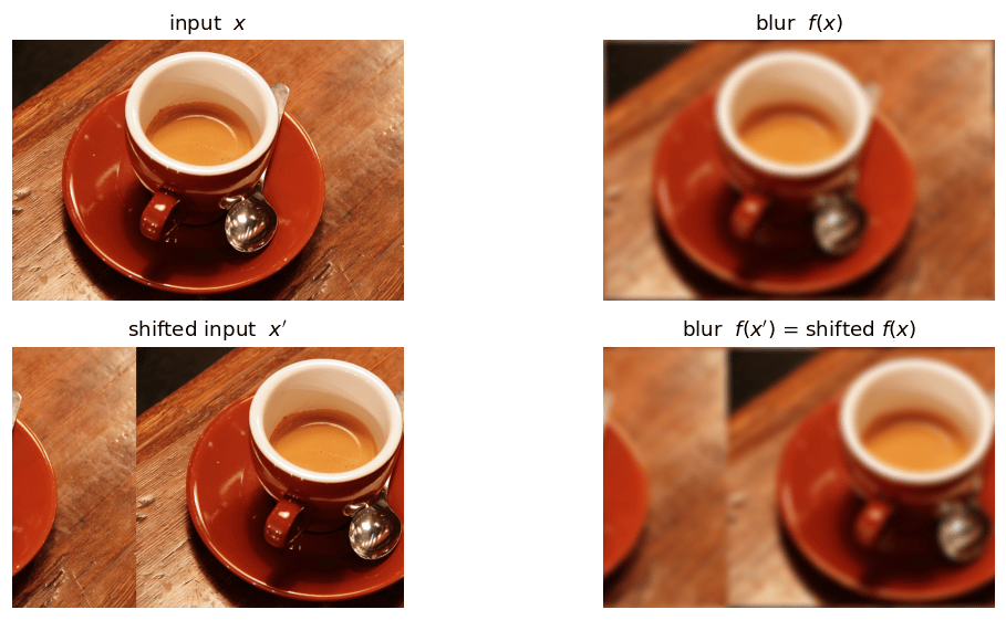
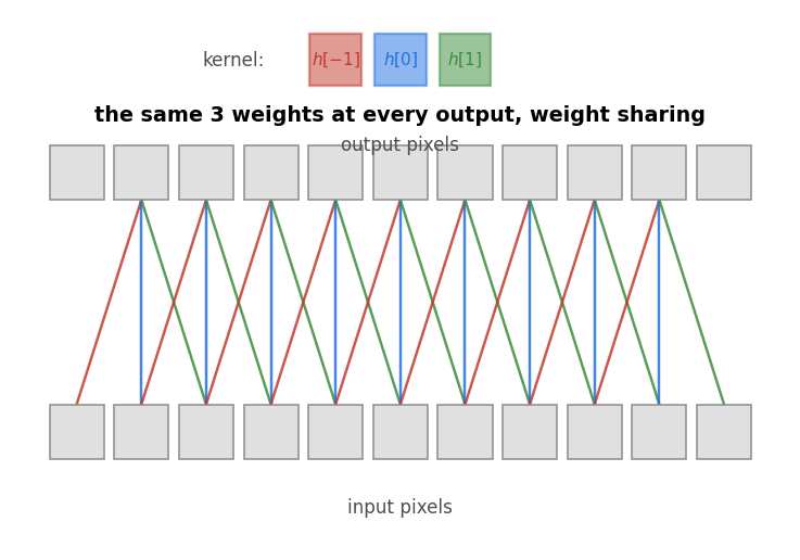
Book Figure 15.7: computed here.
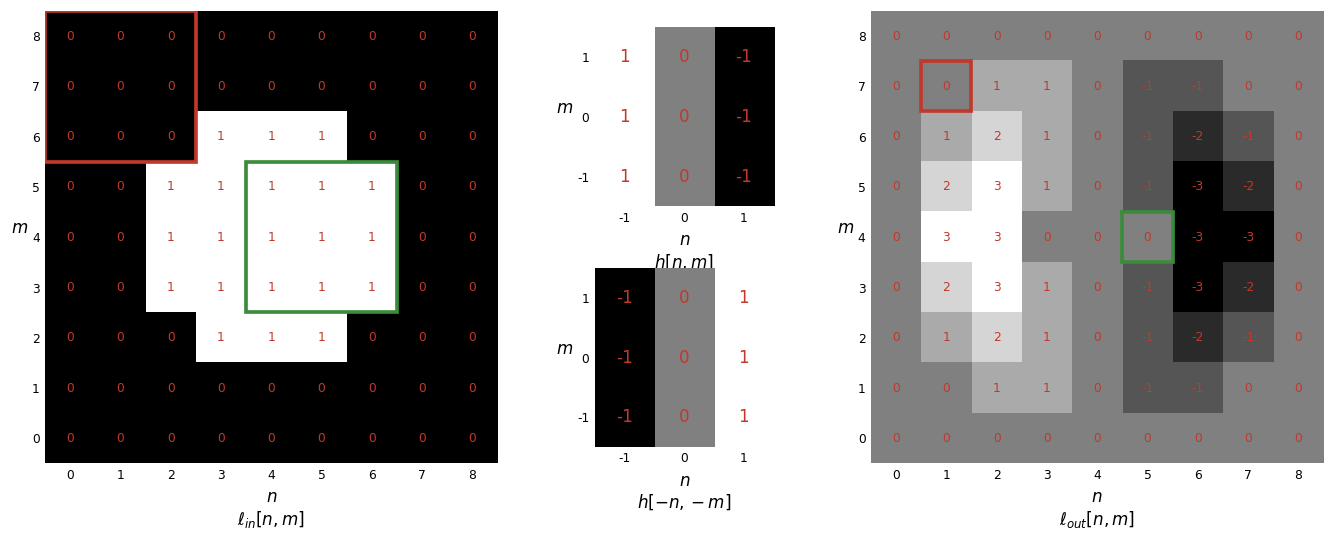
Book Figure 15.8: applied with Kornia.
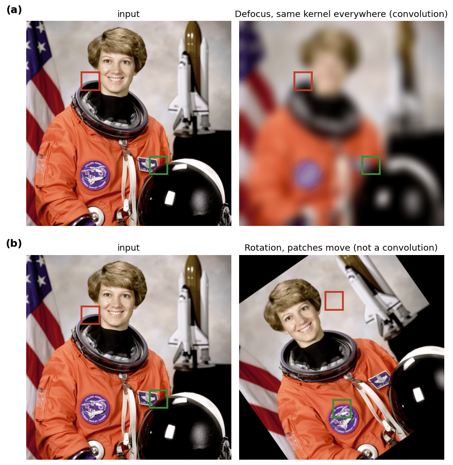
Book Figure 15.9: applied with Kornia.
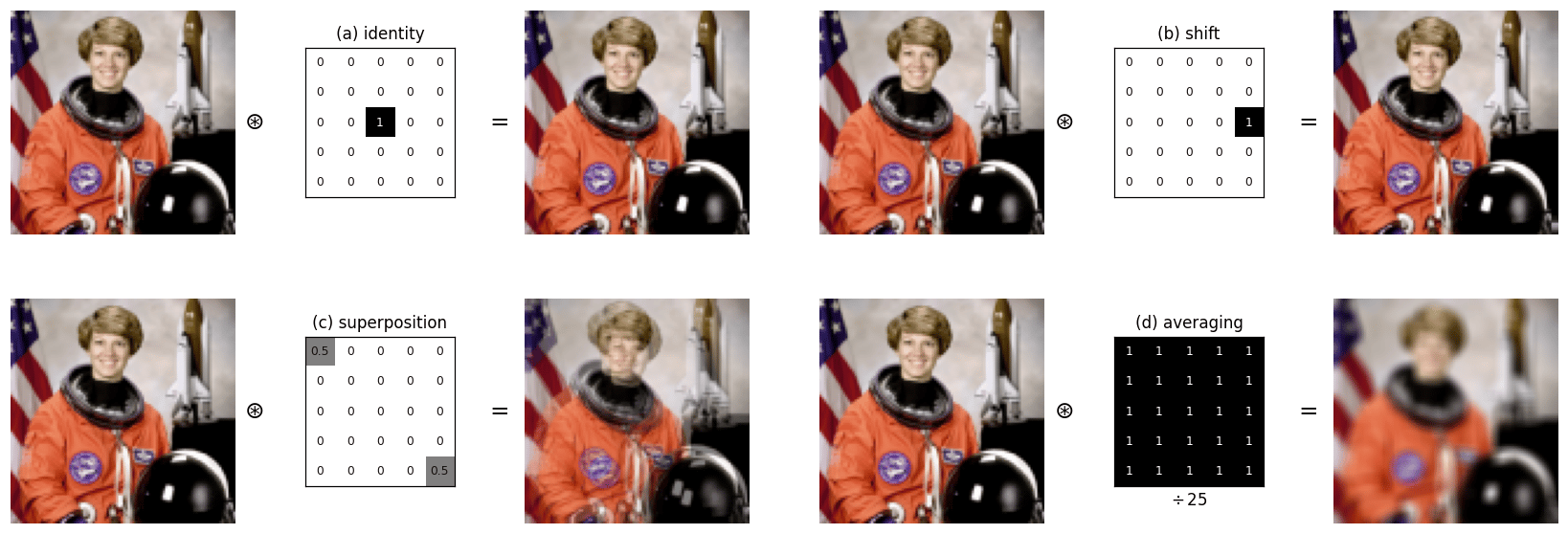
Book Figure 15.10: applied with Kornia.
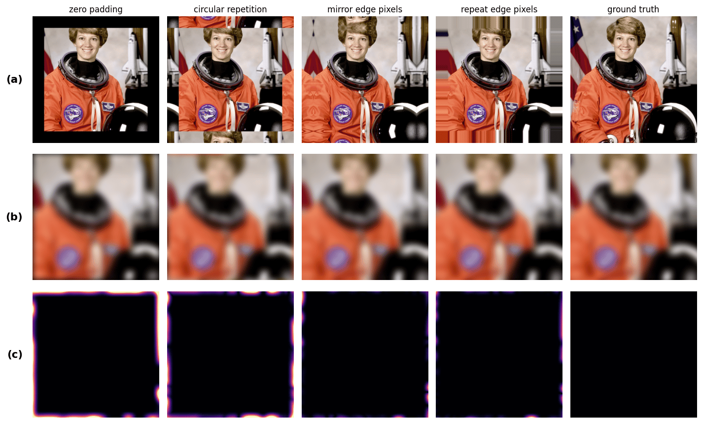
Cross-correlation versus convolution
Cross-correlation is convolution without flipping the kernel. For template matching you slide a template over the image and measure similarity; normalized cross-correlation removes the effect of local brightness. Figure 15.11: cross-correlation vs. convolution (kernel orientation).Book Figure 15.11: computed here.
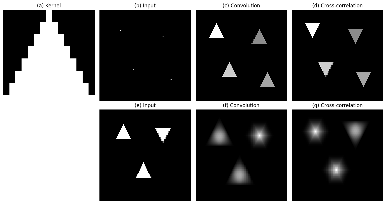
Book Figure 15.12: computed here.

System identification
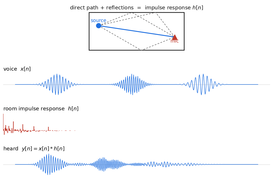
An LTI system is identified by its impulse response: feed in an impulse and read out . A room’s acoustics are an LTI system: a clap measures its impulse response, and any sound is that sound convolved with . Figure 15.13: an LTI system is fully described by its impulse response .Book Figure 15.13: drawn as a schematic.
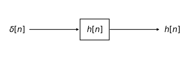
Book Figure 15.16: computed here.
Concluding remarks
Every operation in this section is one idea in different forms. A linear translation-invariant system is a matrix multiply whose matrix is banded and Toeplitz (Figures 15.4 and 15.6). Equivalently, it is a convolution with a single kernel, the impulse response, applied at every position (Figures 15.6 to 15.9). Blurring, shifting, averaging, edge detection, and template matching are all just different kernels. Cross-correlation is the same computation without the flip (Figure 15.11), and with local normalization it becomes a robust template detector (Figure 15.12). Because an LTI system is fully described by its impulse response, you can identify it by measuring that response, whether the system is a lens, a filter, or a room (Figures 15.13 to 15.16).Found an error on this page? Report an issue.