Every method in this chapter treats an image as a function that you can filter, differentiate, and sample. This section fixes what that function is: how pixels are indexed, what values they hold, and how those values are rescaled before any processing.

Grayscale images

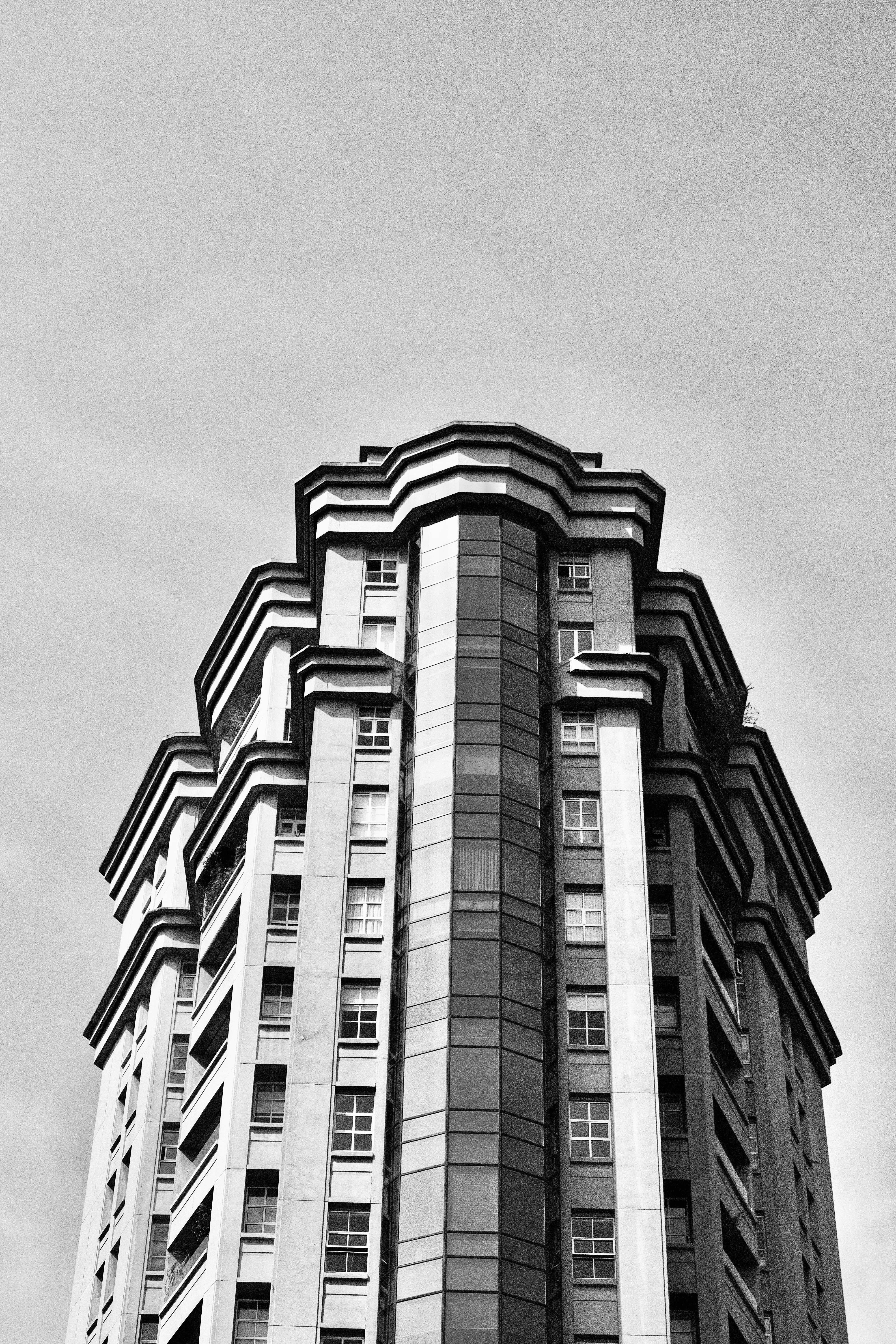
A grayscale photograph A grayscale image is a matrix of pixel intensities. Each pixel holds one value, the light intensity at that point. In an 8-bit encoding the value ranges from 0 (black) to 255 (white). An image of size w×hw \times h has ww columns (its width) and hh rows (its height). You write it as x(i,j)\mathbf x(i,j), where the row index ii runs down the image and the column index jj runs across it. So the column jj corresponds to the horizontal coordinate xx, and the row ii to the vertical coordinate yy. This order, row before column, is the opposite of the (x,y)(x, y) order of plane geometry, and it is a frequent source of bugs. The function f(i,j)f(i,j) maps pixel coordinates to the intensity at that pixel. The sensor’s bit depth sets the dynamic range of the values: [0, 255] for 8 bits, while some cameras capture 10, 12, or 16 bits per pixel.

Color images

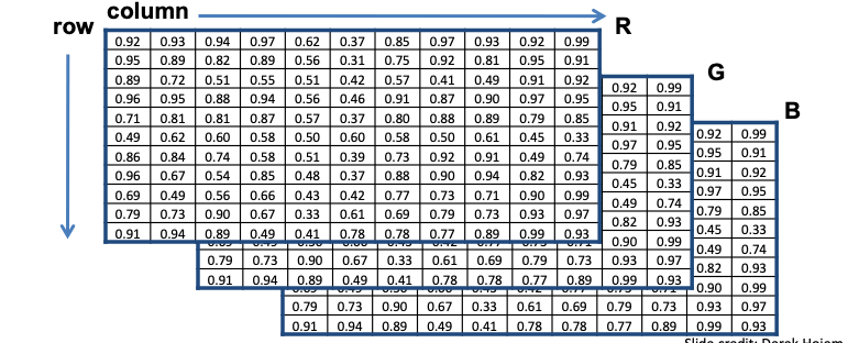
A color image assigns a vector to each pixel instead of a single value: f(i,j)=[r(i,j)g(i,j)b(i,j)]\mathbf f(i,j)= \begin{bmatrix} r(i,j) \\ g(i,j) \\ b(i,j) \end{bmatrix} The third dimension holds the image channels. When the channels are the red, green, and blue primaries, the image is in the RGB color space, and combining the three channels gives the color of each pixel. In code, a color image is therefore a three-dimensional array, and the order of its dimensions is a convention, not something the array enforces. OpenCV, and NumPy code built around it, uses height by width by channels (HWC) and orders the channels blue, green, red. Most PyTorch vision APIs, including the torchvision models, expect channels by height by width (CHW) in red, green, blue order. Converting between the two is up to you: torch.from_numpy keeps the HWC order of an OpenCV image, so you still have to permute the dimensions, for example with permute(2, 0, 1), and swap blue and red.

Normalization

Before processing an image, you convert its pixel values to floating-point numbers in [0, 1] by dividing each value by the largest value its channel can hold. This is normalization. For an 8-bit RGB image: xnorm(i,j)=[r(i,j)255g(i,j)255b(i,j)255]\mathbf x_{norm}(i,j) = \begin{bmatrix} \frac{r(i,j)}{255} \\ \frac{g(i,j)}{255} \\ \frac{b(i,j)}{255} \end{bmatrix} Three stacked matrices of values between 0 and 1, one each for the red, green, and blue channels, indexed by row and column A normalized color image as three stacked matrices, one per channel, each indexed by row and column. Slide credit: Derek Hoiem. With the image a function on a grid of real values, the next section, Convolution and Linear Filters, applies the first and most important operation on it.