What Natural Images Have in Common

This section was written by Kaushik Kachireddy (pull request #79), with help from an AI coding agent (Claude Code) on the code. It reproduces the ideas of Chapter 27 of Foundations of Computer Vision by Antonio Torralba, Phillip Isola, and William T. Freeman. The book’s own figures are not reproduced here, because the book’s license covers only the work in full; links point to them instead. Natural images are a vanishingly small, highly structured corner of the space of all pixel arrays. This section measures that structure and builds generative priors from it: the 1/f power law, sampling clouds from it, why an independent-pixel model fails, the decay of pixel correlations, the heavy-tailed (generalized-Laplacian) statistics of derivatives, and how those priors drive denoising: Wiener filtering, wavelet coring, and non-local means. The book measures these statistics on its own photographs. Here the measurements run on scikit-image test photographs (an astronaut, a rocket, a coffee cup, the cameraman, a cat, a clock, grass, and a Hubble deep field) and on generated images, and each figure links to the book’s version. The statistics are properties of natural images in general, so they come out the same.

import numpy as np
import matplotlib.pyplot as plt
from scipy.special import gamma
from skimage.color import rgb2gray
from skimage.transform import resize

np.random.seed(0)
plt.rcParams.update({'figure.dpi': 130, 'savefig.dpi': 130,
                     'image.cmap': 'gray', 'axes.grid': False})

Images replaced for licensing. The book is published under a CC BY-NC-ND license, which covers only the book as a whole and not its individual images, so this page does not republish the book’s photographs. License-free images stand in for them:

The astronaut, rocket, and coffee photographs (scikit-image) stand in for photographs of the MIT dome, a wheel, and autumn leaves (Figure 27.10).
The cameraman photograph (scikit-image) stands in for a photograph of a street (Figures 27.8 and 27.15).
The chelsea photograph (scikit-image) stands in for a photograph of colorful houses (Figure 27.23).
The clock photograph (scikit-image) stands in for a photograph of a doorway (Figure 27.16).
The grass texture (scikit-image) stands in for a photograph of hair (Figure 27.13).
The cameraman photograph (scikit-image) stands in for a photograph of a building in Barcelona (Figure 27.14).
The Hubble deep field, immunohistochemistry, and colorwheel images (scikit-image) and generated clouds stand in for photographs of stars, clouds, plums, and a cube (Figures 27.6 and 27.12).
Generated images and scikit-image photographs stand in for the book’s eight visual worlds (Figure 27.2).

If you use the book for non-commercial purposes, you can swap the originals back in: each line that loads a stand-in carries the original’s link in a comment.

def to_gray_square(img, size=256):
    """Grayscale, center-crop to square, resize to size x size, in [0,1]."""
    g = rgb2gray(img) if img.ndim == 3 else img
    h, w = g.shape; s = min(h, w)
    g = g[(h - s) // 2:(h - s) // 2 + s, (w - s) // 2:(w - s) // 2 + s]
    return resize(g, (size, size), anti_aliasing=True)


def radial_profile(mag):
    """Angular-averaged radial profile of a 2D (fft-shifted) magnitude image."""
    h, w = mag.shape; cy, cx = h // 2, w // 2
    y, x = np.indices((h, w))
    r = np.sqrt((x - cx)**2 + (y - cy)**2).astype(int)
    tbin = np.bincount(r.ravel(), mag.ravel())
    nr = np.bincount(r.ravel())
    return tbin / np.maximum(nr, 1)


def gen_laplacian(x, r, s=1.0):
    """Generalized Laplacian pdf  exp(-|x/s|^r) / (2 (s/r) Gamma(1/r))."""
    return np.exp(-np.abs(x / s)**r) / (2 * (s / r) * gamma(1.0 / r))

def _kurt(a):
    a = a - a.mean(); return float((a**4).mean() / (a.var()**2 + 1e-12))

from skimage import data, img_as_float

def rgbf(im):
    """float RGB in [0, 1] from a scikit-image array (grayscale is repeated over 3 channels)."""
    im = img_as_float(im).astype(np.float32)
    return np.repeat(im[..., None], 3, -1) if im.ndim == 2 else im[..., :3]

def clouds(size=256, alpha=1.5, seed=0):
    """Color 1/f noise: a random-phase sample per channel (the 'clouds' of 27.11)."""
    g = np.random.default_rng(seed); fy = np.fft.fftfreq(size)[:, None]; fx = np.fft.fftfreq(size)[None, :]
    mag = 1.0 / (1.0 + (size * np.sqrt(fx**2 + fy**2))**alpha)
    out = np.stack([np.real(np.fft.ifft2(mag * np.exp(2j * np.pi * g.random((size, size))))) for _ in range(3)], -1)
    return (out - out.min()) / (np.ptp(out) + 1e-9)

# Test photographs in place of the book's images (see the links next to each figure)
# stand-in for photographs of the MIT dome, a wheel, and autumn leaves in the book; original: https://visionbook.mit.edu/stat_image_models_revised.html#fig-FT_angular_averages
DOME, WHEEL, LEAVES = rgbf(data.astronaut()), rgbf(data.rocket()), rgbf(data.coffee())   # 27.10
# stand-in for a photograph of a street in the book; original: https://visionbook.mit.edu/stat_image_models_revised.html#fig-correlation
STREET = rgbf(data.camera())            # grayscale scene (27.8, 27.15)
# stand-in for a photograph of colorful houses in the book; original: https://visionbook.mit.edu/stat_image_models_revised.html#fig-nlm2
BURANO = rgbf(data.chelsea())           # color scene for non-local means (27.23)
# stand-in for a photograph of a doorway in the book; original: https://visionbook.mit.edu/stat_image_models_revised.html#fig-derivativesdistributions
BUILDING = rgbf(data.clock())           # grayscale object photo (27.16)
# stand-in for a photograph of hair in the book; original: https://visionbook.mit.edu/stat_image_models_revised.html#fig-hair
HAIR = rgbf(data.grass())               # oriented texture, in place of hair (27.13, 27.16)
# stand-in for a photograph of a building in Barcelona in the book; original: https://visionbook.mit.edu/stat_image_models_revised.html#fig-denoisingGaussianModel
BCN = rgbf(data.camera())               # grayscale scene for Wiener denoising (27.14)
# stand-in for photographs of stars, clouds, plums, and a cube in the book; original: https://visionbook.mit.edu/stat_image_models_revised.html#fig-histMatch
STARS = rgbf(data.hubble_deep_field())[:400, :400]    # a real star field (27.6, 27.12)
CLOUDS = clouds()                                      # generated clouds (27.6, 27.12)
PLUMS = rgbf(data.immunohistochemistry())              # blob-like color image (27.6, 27.12)
CUBE = rgbf(data.colorwheel())                         # smooth color structure (27.6, 27.12)
print('street', STREET.shape, ' stars', STARS.shape, ' clouds', CLOUDS.shape)

street (512, 512, 3)  stars (400, 400, 3)  clouds (256, 256, 3)

The 1/f power law

The single most robust statistic of natural images: the Fourier magnitude falls off as a power law in radial frequency,

\lVert\mathscr L(u,v)\rVert \;\simeq\; \frac{1}{w^{\alpha}},\qquad w=\sqrt{u^2+v^2},\ \ \alpha\approx 1\text{ to }1.5.

Three real photos concentrate their energy (the book’s version is Figure 27.10) at low frequency and their angular-averaged spectra hug the

1/w^{1.5}

curve; white noise is flat: no power law at all.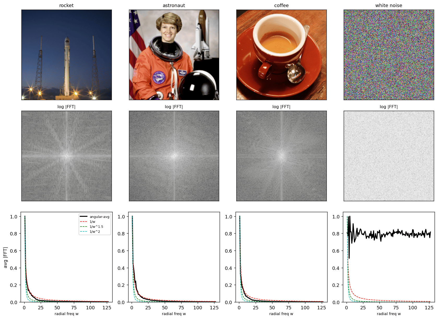

# Figure 27.10: images (top, COLOR as in the book), |FFT| (mid), radial spectra (bottom).
def sq_col(img, size=256):
    h, w = img.shape[:2]; s = min(h, w)
    c = img[(h - s) // 2:(h - s) // 2 + s, (w - s) // 2:(w - s) // 2 + s]
    return resize(c, (size, size), anti_aliasing=True)

noise_rgb = np.random.rand(256, 256, 3)                       # color white noise (book uses RGB)
imgs = [('rocket', sq_col(WHEEL)), ('astronaut', sq_col(DOME)),
        ('coffee', sq_col(LEAVES)), ('white noise', noise_rgb)]

Sampling from the power spectrum

A Gaussian image prior with a

1/(1+w^{\alpha})

power spectrum is easy to sample: take that magnitude, attach random phase, and inverse-transform. The result has the right spectral falloff but no real structure: it always looks like clouds, in grayscale or (sampling each channel) in color.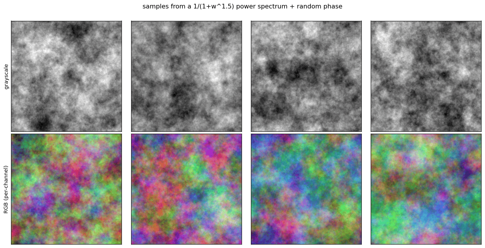

# Figure 27.11: cloud samples from a 1/(1+w^1.5) spectrum, gray (top) + RGB (bottom).
def one_over_f_sample(size=256, alpha=1.5, rng=None):
    rng = rng or np.random
    fy = np.fft.fftfreq(size)[:, None]; fx = np.fft.fftfreq(size)[None, :]
    w = np.sqrt(fx**2 + fy**2); mag = 1.0 / (1.0 + (size * w)**alpha)
    phase = np.exp(2j * np.pi * rng.rand(size, size))
    img = np.real(np.fft.ifft2(mag * phase))
    return (img - img.min()) / (np.ptp(img) + 1e-9)

The independent-pixel model

The simplest model treats every pixel as an independent draw from one histogram. Sampling from it keeps the image’s color and intensity distribution exactly but destroys all spatial arrangement: the sample is just noise with the right histogram. It only ever looks right for images that are essentially unstructured, like a star field. The book’s version is Figure 27.6.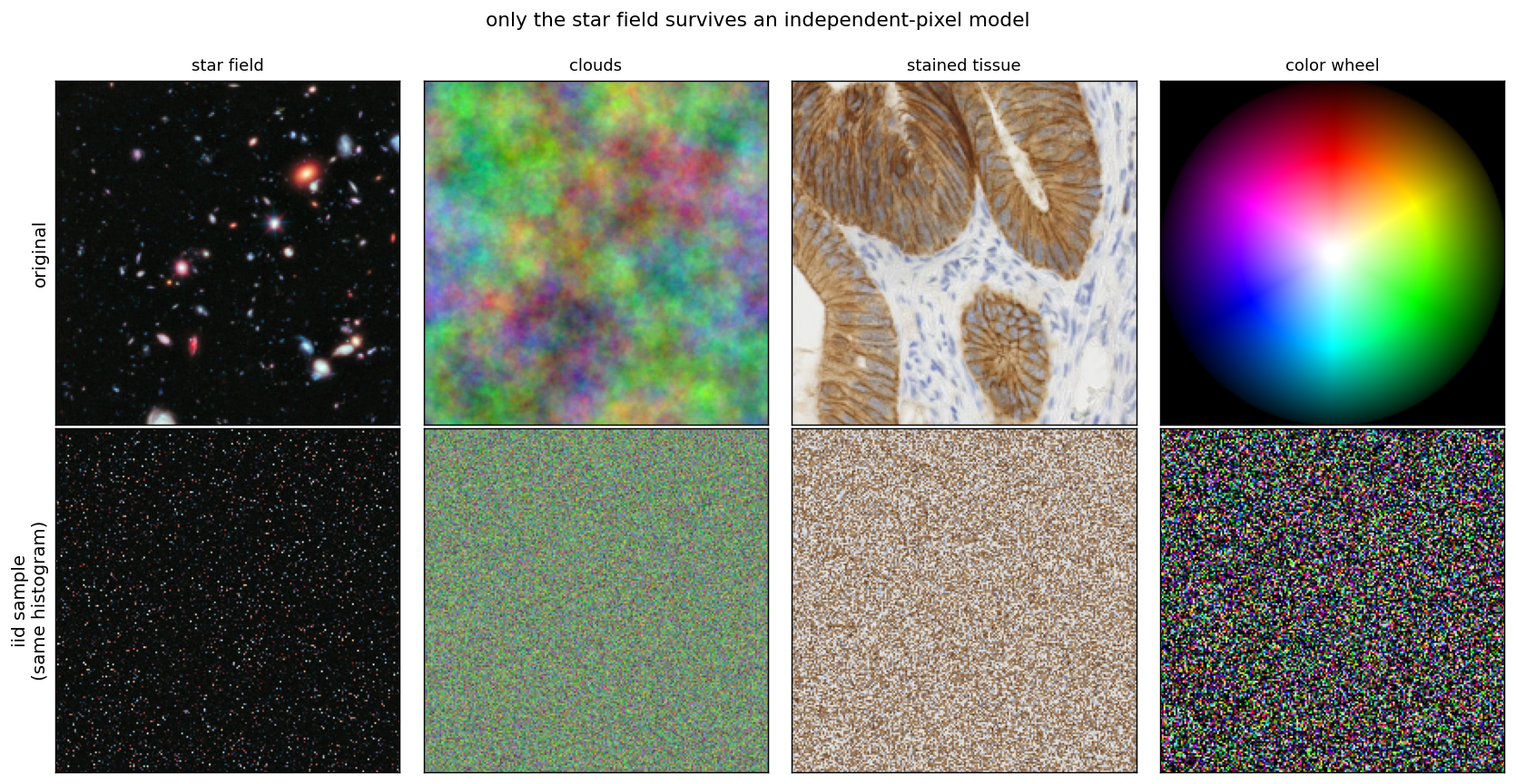

# Figure 27.6: original (top) vs independent-pixel sample (bottom), four
# images. An iid draw from the exact color histogram = a random shuffle of
# the pixels: same histogram, all structure gone.
def iid_sample(img):
    flat = img.reshape(-1, img.shape[-1])
    return flat[np.random.permutation(len(flat))].reshape(img.shape)

def sq(img, size=200):
    h, w = img.shape[:2]; s = min(h, w)
    return resize(img[(h - s) // 2:(h - s) // 2 + s, (w - s) // 2:(w - s) // 2 + s],
                  (size, size), anti_aliasing=True)

pics = [('star field', sq(STARS)), ('clouds', sq(CLOUDS)),
        ('stained tissue', sq(PLUMS)), ('color wheel', sq(CUBE))]

Pixel correlations decay with distance

Neighboring pixels are highly correlated; the correlation falls as they move apart. Scatter plots of

\ell[n]

\ell[n+d]

tighten around the diagonal for small

d

and spread out for large

d

(the book’s version is Figure 27.8).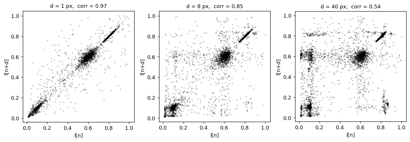

# Figure 27.8: pixel-pair scatter at increasing horizontal distance d.
g = to_gray_square(STREET, 256)

Derivatives are heavy-tailed, not Gaussian

The histogram of raw intensities is broad and near-uniform, but the histogram of image derivatives is sharply peaked at zero with heavy tails: most of an image is smooth (derivative

\approx 0

) with rare large jumps at edges. On a log scale the derivative histogram is a cusp, nothing like a parabola (Gaussian).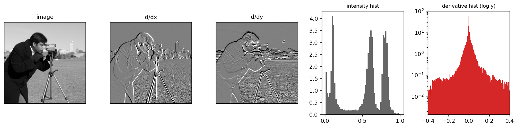

# Figure 27.15: image, dx, dy, and the intensity vs derivative histograms.
g = to_gray_square(STREET, 256)
dx = g[:, 1:] - g[:, :-1]
dy = g[1:, :] - g[:-1, :]

print('kurtosis  intensity: %.1f   derivative: %.1f  (Gaussian = 3)'
      % (_kurt(g.ravel()), _kurt(dx.ravel())))

kurtosis  intensity: 1.7   derivative: 27.1  (Gaussian = 3)

The generalized Laplacian

Derivative statistics are fit by the generalized Laplacian

p(x)\propto \exp\!\big(-|x/s|^{\,r}\big),

with

r\!=\!2

Gaussian,

r\!=\!1

Laplacian, and $r\in[0.4,0.8]$ for natural images: sharper peak, heavier tails than a Gaussian.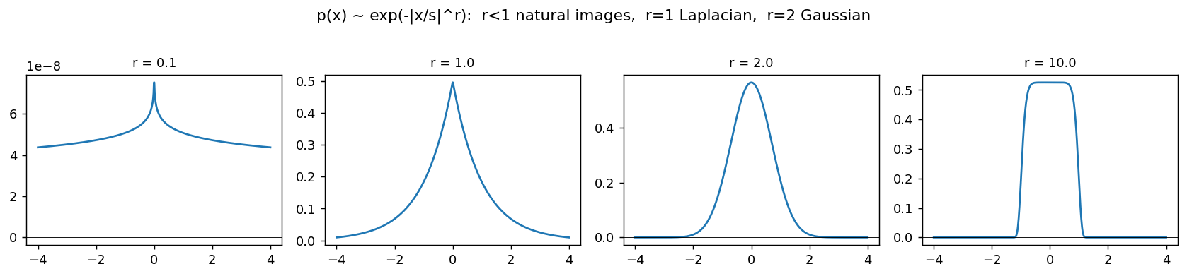

# Figure 27.17: generalized-Laplacian shapes for r = 0.1, 1, 2, 10.
x = np.linspace(-4, 4, 600)

[1,-1] statistics: noise stays Gaussian, images do not

Following the book (Figure 27.16), three ‘visual worlds’, Gaussian noise, a photograph of a clock, and a grass texture, are each shown with the image, its intensity histogram, its

[1,-1]

derivative, and the derivative histogram (red) with the best Gaussian fit (black). The derivative of noise stays Gaussian; both photographs give the same sharply peaked, heavy-tailed shape that the Gaussian fit misses.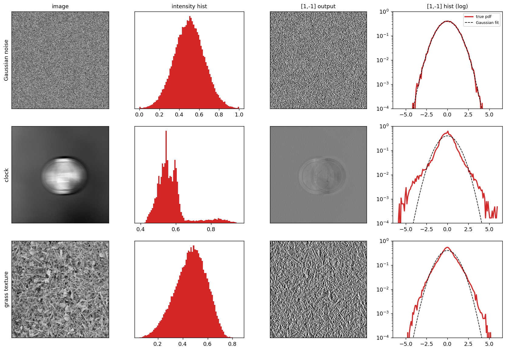

# Figure 27.16: image | intensity hist | [1,-1] output | output hist, x 3 worlds.
worlds = [('Gaussian noise', np.clip(0.5 + 0.15 * np.random.randn(256, 256), 0, 1)),
          ('clock', to_gray_square(BUILDING)),
          ('grass texture', to_gray_square(HAIR))]

Denoising with the Gaussian (1/f) prior: the Wiener filter

Under a Gaussian prior with power spectrum

S(w)=A/w^{2\alpha}

and white noise of variance

\sigma^2

, the MAP estimate is the Wiener filter

\mathscr L(w)=\frac{S(w)}{S(w)+\sigma^2}\,\mathscr L_g(w),

which keeps low frequencies (where the image dominates) and suppresses high frequencies (where noise dominates). The book’s version is Figure 27.14.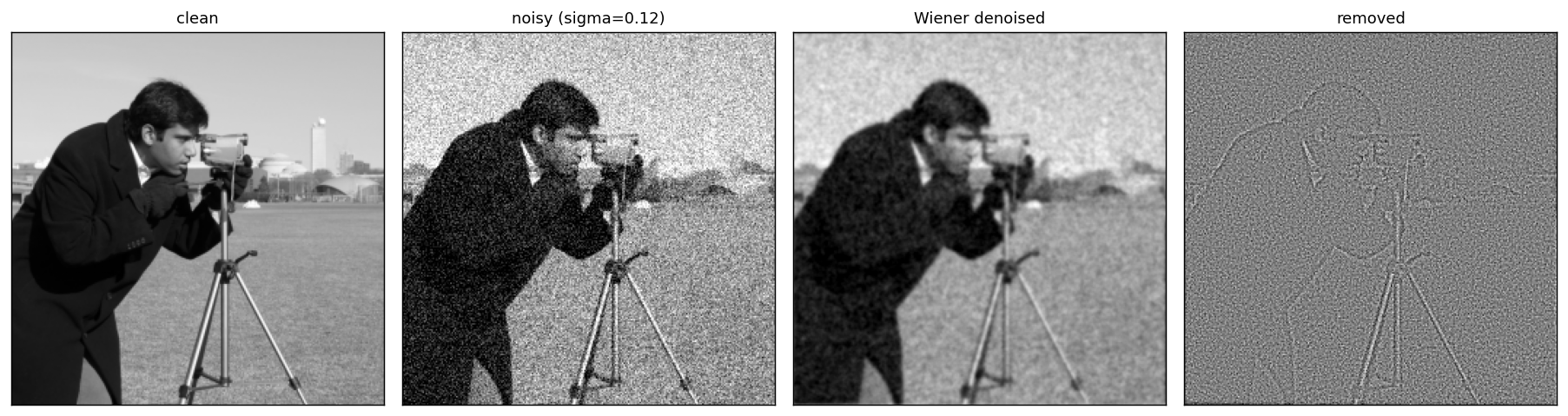

# Figure 27.14: clean, noisy, Wiener-denoised, and the removed noise.
g = to_gray_square(BCN, 256); sigma = 0.12
noisy = g + sigma * np.random.randn(*g.shape)
fy = np.fft.fftfreq(256)[:, None]; fx = np.fft.fftfreq(256)[None, :]
w = np.sqrt(fx**2 + fy**2) * 256 + 1e-3                   # fftfreq order (unshifted)
# Wiener gain  S/(S+sigma^2) for a 1/f^{2a} prior S = A/w^{2a}; writing A via the
# crossover w0 where signal power = noise power gives  H = 1/(1 + (w/w0)^{2a}).
alpha, w0 = 1.5, 45.0
H = 1.0 / (1.0 + (w / w0)**(2 * alpha))
den = np.real(np.fft.ifft2(np.fft.fft2(noisy - noisy.mean()) * H)) + noisy.mean()
show = [(g, 'clean'), (noisy, 'noisy (sigma=0.12)'), (den, 'Wiener denoised'), (0.5 + (noisy - den), 'removed')]

print('RMSE  noisy: %.4f   denoised: %.4f' % (np.sqrt(((noisy - g)**2).mean()), np.sqrt(((den - g)**2).mean())))

RMSE  noisy: 0.1201   denoised: 0.0500

Wavelet denoising as coring

With a Laplacian prior on a band-pass coefficient and Gaussian noise, the MAP estimate shrinks small coefficients toward zero and leaves large ones almost untouched: a coring curve. Small (probably-noise) responses are cored out; strong (probably-signal) responses survive.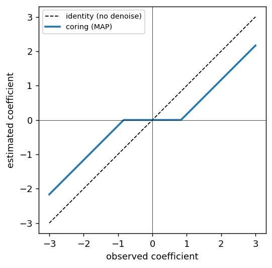

# Figure 27.21: the coring (shrinkage) curve for a Laplacian prior.
def coring(xhat, s=0.3, sigma=0.5):
    # MAP of  p(x) ~ exp(-|x|/s) * exp(-(x-xhat)^2/2sigma^2): soft-threshold by sigma^2/s.
    t = sigma**2 / s
    return np.sign(xhat) * np.maximum(np.abs(xhat) - t, 0.0)

xhat = np.linspace(-3, 3, 400)

Non-local means

Rather than a parametric prior, non-local means denoises each pixel by averaging other pixels whose surrounding patch looks similar: a nonparametric image model. It exploits the self-similarity (repeated structure) of natural images. The book’s version is Figure 27.23.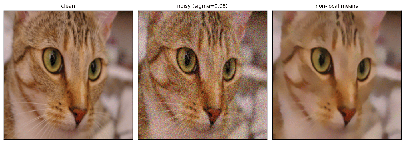

# Figure 27.23: clean, noisy, and non-local-means denoised (a color photo,
# shown full-frame, not center-cropped).
from skimage.restoration import denoise_nl_means
g = resize(BURANO, (232, 232), anti_aliasing=True)         # full color scene
sigma = 0.08
noisy = np.clip(g + sigma * np.random.randn(*g.shape), 0, 1)
nlm = denoise_nl_means(noisy, h=0.8 * sigma, sigma=sigma, patch_size=5,
                       patch_distance=6, fast_mode=True, channel_axis=-1)

print('RMSE  noisy: %.4f   NLM: %.4f' % (np.sqrt(((noisy - g)**2).mean()), np.sqrt(((nlm - g)**2).mean())))

RMSE  noisy: 0.0794   NLM: 0.0309

More representations from the chapter

The figures above cover the chapter’s core arc. Below are several more of the book’s representations that are worth reproducing: the space of visual worlds (27.2), the dead-leaves generative model (27.9), the role of Fourier phase (27.12), a Gaussian texture model (27.13), and how the prior shapes reconstruction (27.19) and wavelet coefficient estimation (27.20).

Eight visual worlds

Different sources of images (noise, an oriented Gabor, a Mondrian, a star field, clouds, lines, rendered graphics, a photograph) occupy very different regions of image space, each with its own statistics. A single model cannot fit them all. The book’s version is Figure 27.2; here the eight are generated or taken from test images.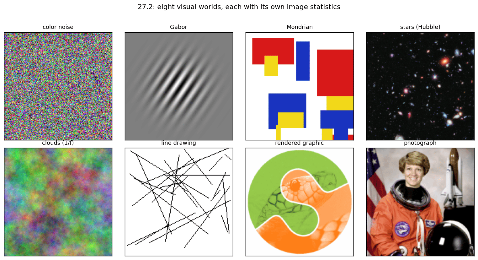

from skimage.draw import line
g = np.random.default_rng(0); S = 160
yy, xx = np.mgrid[0:S, 0:S] / S
# stand-in for the eight visual worlds in the book; original: https://visionbook.mit.edu/stat_image_models_revised.html#fig-worlds
noise = g.random((S, S, 3))
gab = 0.5 + 0.5 * np.cos(2 * np.pi * 12 * (xx * np.cos(0.6) + yy * np.sin(0.6))) * np.exp(-((xx - .5)**2 + (yy - .5)**2) / 0.05)
mondrian = np.ones((S, S, 3))
palette = np.array([[.85, .1, .1], [.1, .2, .75], [.95, .85, .1], [1, 1, 1], [.05, .05, .05]])
for _ in range(16):
    y0, x0 = g.integers(0, S, 2); h, w = g.integers(15, 70, 2)
    mondrian[y0:y0 + h, x0:x0 + w] = palette[g.integers(len(palette))]
drawing = np.ones((S, S, 3))
for _ in range(25):
    r0, c0, r1, c1 = g.integers(0, S, 4); rr, cc = line(r0, c0, r1, c1); drawing[rr, cc] = 0
logo = img_as_float(data.logo()); cgi = logo[..., :3] * logo[..., 3:] + (1 - logo[..., 3:])   # rendered graphic on white
worlds = [(noise, 'color noise'), (np.repeat(gab[..., None], 3, -1), 'Gabor'),
          (mondrian, 'Mondrian'), (resize(STARS, (S, S, 3)), 'stars (Hubble)'),
          (resize(CLOUDS, (S, S, 3)), 'clouds (1/f)'), (drawing, 'line drawing'),
          (resize(cgi, (S, S, 3)), 'rendered graphic'), (resize(DOME, (S, S, 3)), 'photograph')]

The dead-leaves model

A simple generative model of natural images: repeatedly drop opaque colored shapes (disks and squares) of random size, each occluding what is beneath. Like the book (Figure 27.9), the figure shows a disk version and a square version. Occlusion alone reproduces hallmarks of natural-image statistics: scale-invariant structure and a heavy-tailed derivative histogram.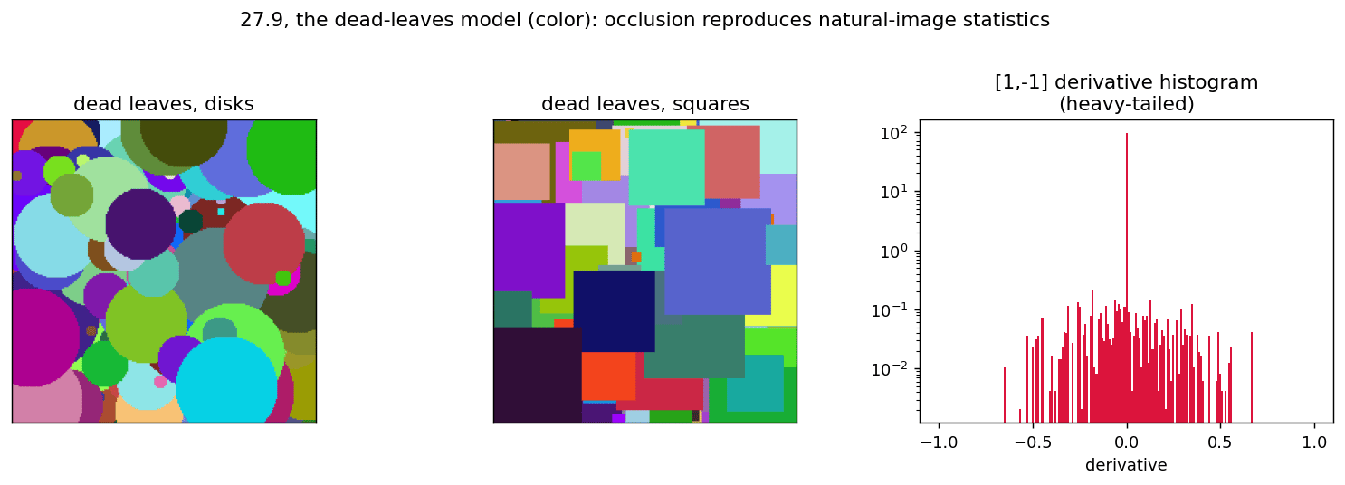

def dead_leaves(size=220, n=1600, rmin=3, rmax=40, seed=0, squares=False):
    g = np.random.default_rng(seed); img = np.full((size, size, 3), 0.5)
    yy, xx = np.mgrid[0:size, 0:size]
    for _ in range(n):
        cx, cy = g.integers(0, size, 2); r = g.integers(rmin, rmax); col = g.random(3)
        m = (np.abs(xx-cx) < r) & (np.abs(yy-cy) < r) if squares else ((xx-cx)**2 + (yy-cy)**2 < r*r)
        img[m] = col
    return img
dl_c = dead_leaves(seed=1); dl_s = dead_leaves(seed=2, squares=True)

Matched Fourier magnitude: phase carries the structure

The 1/f power spectrum (27.10) fixes the Fourier magnitude. But the magnitude alone does not make an image look like anything: keep each image’s magnitude and replace its phase with random phase, and the recognizable content dissolves into 1/f texture. It is the phase that encodes edges and objects. The book’s version is Figure 27.12.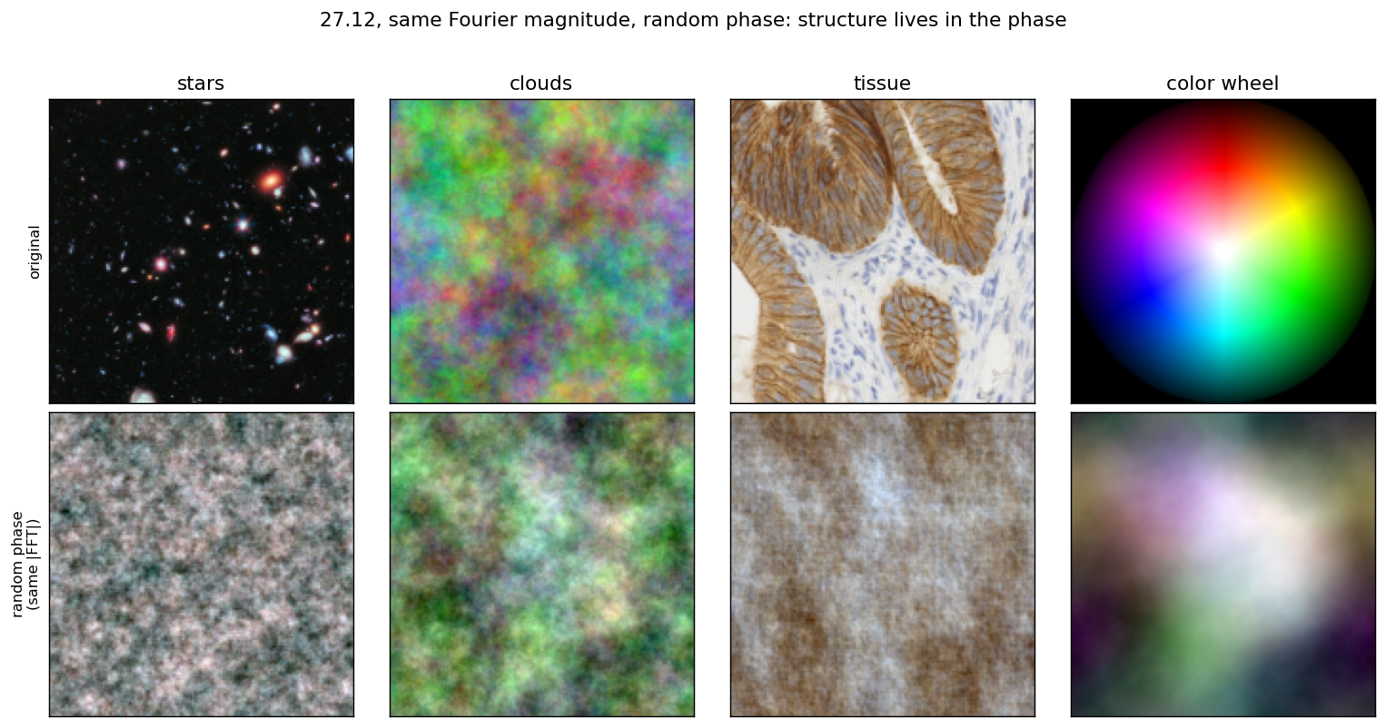

def random_phase(img):
    ph = np.angle(np.fft.fft2(np.random.default_rng(0).standard_normal(img.shape[:2])))  # one phase field, shared across color
    out = np.zeros_like(img)
    for c in range(img.shape[2]):
        mag = np.abs(np.fft.fft2(img[..., c]))
        out[..., c] = np.fft.ifft2(mag * np.exp(1j*ph)).real
    return np.clip((out - out.min()) / (np.ptp(out) + 1e-9), 0, 1)
pairs = [('stars', STARS), ('clouds', CLOUDS), ('tissue', PLUMS), ('color wheel', CUBE)]

A Gaussian texture model

The fully second-order (Gaussian) model of a texture keeps only the mean and the power spectrum, and draws a sample with random phase. The book shows this on hair; here it runs on grass, another oriented texture. The model captures the dominant orientation and scale, but having thrown away the phase, it cannot reproduce the individual blades; the sample looks like a phase-scrambled version.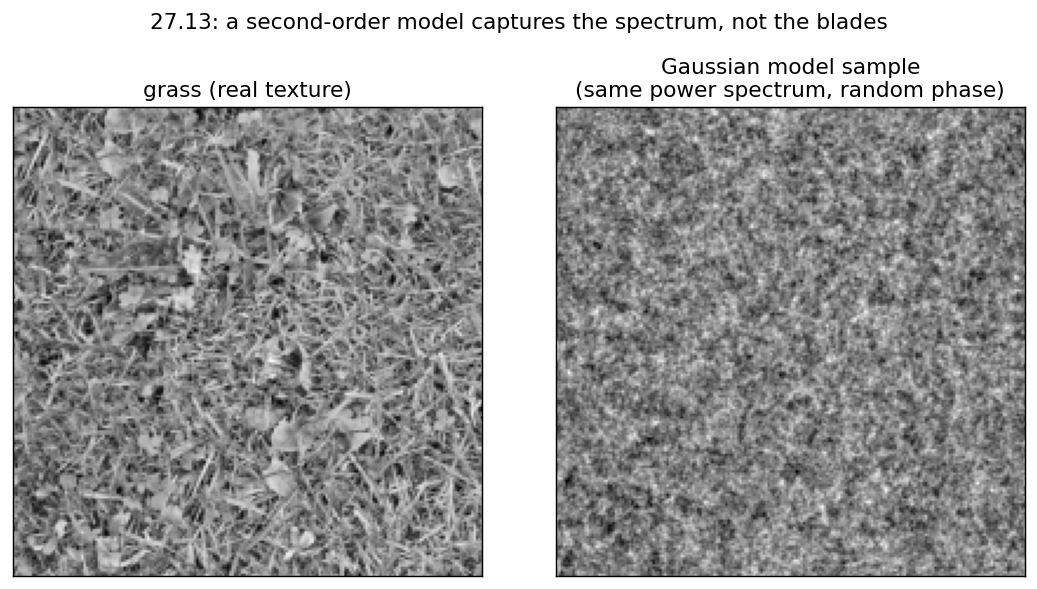

hair = to_gray_square(HAIR, 200)
F = np.fft.fft2(hair - hair.mean()); mag = np.abs(F)
ph = np.angle(np.fft.fft2(np.random.default_rng(3).standard_normal(hair.shape)))
sample = hair.mean() + np.fft.ifft2(mag * np.exp(1j*ph)).real

The prior decides how a reconstruction looks

Reconstructing a 1-D signal from noisy samples: a Gaussian (L2) smoothness prior penalizes all differences quadratically and rounds off the edges; a heavy-tailed (total-variation) prior tolerates a few large jumps, so it keeps edges sharp while flattening the noise: the 1-D analogue of edge-preserving image denoising.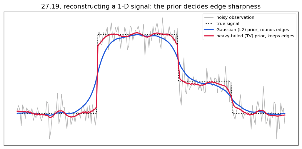

from numpy.fft import rfft, irfft
from skimage.restoration import denoise_tv_chambolle
g = np.random.default_rng(1); n = 200
sig = np.zeros(n); sig[60:120] = 1.0; sig[120:160] = 0.4
obs = sig + 0.12 * g.standard_normal(n)
w = 2*np.pi*np.fft.rfftfreq(n); l2 = irfft(rfft(obs)/(1 + 40.0*w**2), n)   # Gaussian (L2) prior
tv = denoise_tv_chambolle(obs, weight=0.4)                                 # heavy-tailed (TV) prior

Prior × likelihood = posterior for a wavelet coefficient

Estimating a single band-pass (wavelet) coefficient from a noisy measurement: the heavy-tailed prior (peaked at 0) multiplied by the Gaussian likelihood (centered on the noisy observation) gives a posterior whose peak is pulled back toward zero. Small coefficients are shrunk to (near) zero and large ones are kept: exactly the coring nonlinearity of 27.21.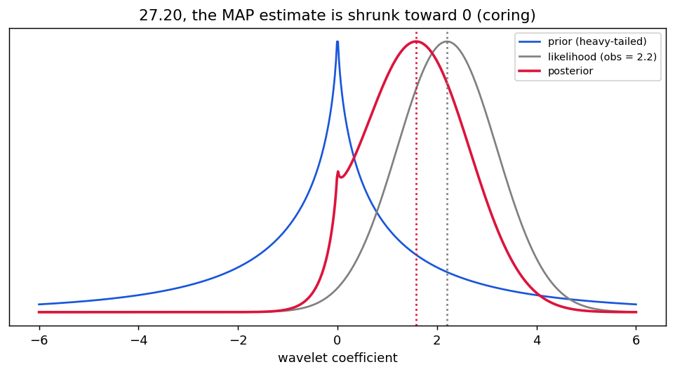

x = np.linspace(-6, 6, 600); y_obs = 2.2; sigma = 1.0
prior = gen_laplacian(x, r=0.6, s=0.7); prior /= prior.max()
like = np.exp(-(x - y_obs)**2 / (2*sigma**2)); like /= like.max()
post = prior * like; post /= post.max()

Concluding remarks

Statistic / model	What it captures	Use
$1/w^{\alpha}$ power law	second-order (Fourier) structure	Gaussian prior, Wiener denoising
pixel-correlation decay	short-range dependence	why iid pixels fail
generalized Laplacian of derivatives	heavy tails / sparsity	wavelet coring
non-local self-similarity	repeated structure	non-local means

Natural images occupy a tiny, structured sliver of image space. Measuring that structure, a power law here, heavy-tailed derivatives there, gives priors that turn ill-posed problems (denoising, inpainting, super-resolution) into tractable Bayesian estimates, and sets the stage for the learned generative models later in the book.

Edit this page on GitHub or file an issue.

Perception

Image Processing

CNNs

Scene Understanding

Faster RCNN Lab

YOLO Lab

UNet Lab

Mask RCNN Lab

What Natural Images Have in Common

The 1/f power law

Sampling from the power spectrum

The independent-pixel model

Pixel correlations decay with distance

Derivatives are heavy-tailed, not Gaussian

The generalized Laplacian

[1,-1] statistics: noise stays Gaussian, images do not

Denoising with the Gaussian (1/f) prior: the Wiener filter

Wavelet denoising as coring

Non-local means

More representations from the chapter

Eight visual worlds

The dead-leaves model

Matched Fourier magnitude: phase carries the structure

A Gaussian texture model

The prior decides how a reconstruction looks

Prior × likelihood = posterior for a wavelet coefficient

Concluding remarks

​The 1/f power law

​Sampling from the power spectrum

​The independent-pixel model

​Pixel correlations decay with distance

​Derivatives are heavy-tailed, not Gaussian

​The generalized Laplacian

​[1,-1] statistics: noise stays Gaussian, images do not

​Denoising with the Gaussian (1/f) prior: the Wiener filter

​Wavelet denoising as coring

​Non-local means

​More representations from the chapter

​Eight visual worlds

​The dead-leaves model

​Matched Fourier magnitude: phase carries the structure

​A Gaussian texture model

​The prior decides how a reconstruction looks

​Prior × likelihood = posterior for a wavelet coefficient

​Concluding remarks

The 1/f power law

Sampling from the power spectrum

The independent-pixel model

Pixel correlations decay with distance

Derivatives are heavy-tailed, not Gaussian

The generalized Laplacian

[1,-1] statistics: noise stays Gaussian, images do not

Denoising with the Gaussian (1/f) prior: the Wiener filter

Wavelet denoising as coring

Non-local means

More representations from the chapter

Eight visual worlds

The dead-leaves model

Matched Fourier magnitude: phase carries the structure

A Gaussian texture model

The prior decides how a reconstruction looks

Prior × likelihood = posterior for a wavelet coefficient

Concluding remarks