


Free energy as the selecting principle
The Fokker-Planck section measured the Ornstein-Uhlenbeck density path and found that it is not the geodesic between its endpoints. Its normalized action is almost four times , so least action does not select it. This section names the principle that does: the path descends a free energy as steeply as the Wasserstein geometry allows. You first see this on Gaussians, where the geometry is an ordinary plane and the descent can be drawn. The same statement then carries over to all densities on the line, where it can be solved one implicit step at a time. The running example is the one of the Fokker-Planck section: the three-component mixture , the forward process , and the horizon . The density is a closed-form mixture, and the score is a responsibility-weighted sum of component scores. Free energies, actions and Fisher information come from quadrature, the Gaussian gradient flow from an ordinary differential equation solver, and the implicit steps from numerical optimization.Gradient descent and its implicit step
Gradient flow moves a point downhill on a function with . Its implicit Euler step with time step is Setting the gradient of the right side to zero gives , the backward Euler update. The minimization uses only the function and the distance, so the step can be written on any space that has a distance, including a space of probability densities with the distance .Gaussians as a plane
For two Gaussians on the line the Wasserstein distance has a closed form, The family of Gaussians is therefore the half plane of points with , and is the ordinary Euclidean distance in that plane. Geodesics are straight segments. Take as free energy the KL divergence to the standard normal . On Gaussians it is with its minimum at . The gradient is , so the gradient flow in the plane is Its solution is and . These are the mean and the standard deviation of the Ornstein-Uhlenbeck process started from , whose variance is . The process maps Gaussians to Gaussians, so on this family it is the gradient flow of the KL divergence in the plane. To check this, the gradient flow is integrated numerically from over and compared with the closed-form Ornstein-Uhlenbeck moments.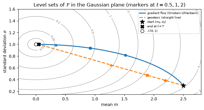
Free energy on densities
The free energy of a density on the line is the KL divergence to , The first term is the negative entropy and the second a potential energy. The constant has no effect on the flow. For a Gaussian, reduces to the formula of the plane. In one dimension the quantile function turns all three ingredients into simple integrals over . Substitute . Then and , so The last line says that is the ordinary distance between quantile functions. A Wasserstein gradient flow on the line is therefore an ordinary gradient flow of , written as a functional of on the set of increasing functions (Santambrogio, 2015). The plane of Gaussians is the special case , with the standard normal CDF. The same flow can be written on the density. The first variation of is . A Wasserstein gradient flow moves mass with the velocity of the first variation, so This is the probability flow velocity of the Fokker-Planck section. The continuity equation with this velocity is , the Fokker-Planck equation of the Ornstein-Uhlenbeck process. The density path of diffusion is the Wasserstein gradient flow of the KL divergence to its equilibrium. All quantile computations on this page use one grid of levels. The levels are with equally spaced, which puts more levels in the tails. On that grid, is the finite difference on each interval and the integrals use the trapezoid rule.Dissipation equals action
Along the flow the free energy falls at a rate fixed by the velocity. Differentiate in time, substitute the continuity equation, and integrate by parts: Since , the last integral is the relative Fisher information . Integrating from to gives the physical-time action of the Fokker-Planck section. The Benamou-Brenier formula bounds by the normalized action (Benamou & Brenier, 2000), so Numerically, comes from quadrature on with computed by log-sum-exp. Its time derivative comes from central differences with step , at 41 times in , and is compared with the Fisher information computed from the exact velocity. The action integrates the Fisher information over 801 times, spaced more densely near .The JKO step
The implicit step of the first table, written with and , is the JKO step (Jordan et al., 1998): Jordan, Kinderlehrer and Otto proved that as these steps converge to the solution of the Fokker-Planck equation. Each step trades a lower free energy against the cost of moving mass, without using a velocity or a score. On the line the step is a minimization over quantile functions, Every experiment uses the same discretization on the grid above. The unknowns are and the logarithms of the spacings , so the computed is increasing by construction. In these variables the entropy term is linear. The minimization uses L-BFGS with the exact gradient, warm-started from the previous step. The error of step is the distance on the grid between and the exact quantile function at time . The first test starts from the Gaussian , where the exact answer is from the plane. It runs to with and .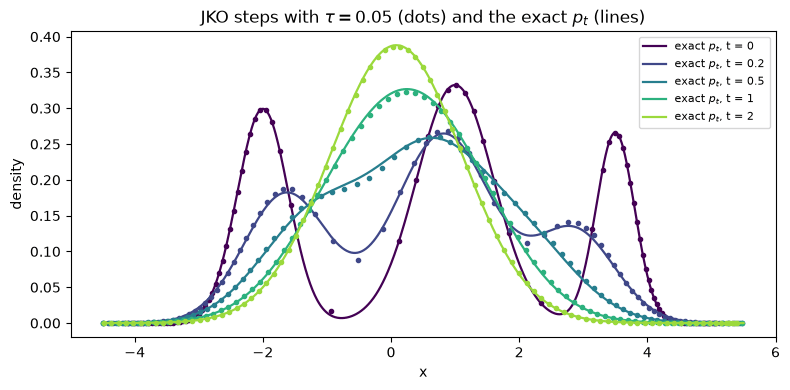
Geodesic or gradient flow
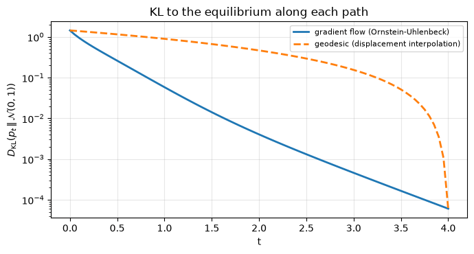
The plane of Gaussians showed two paths between the same endpoints. The same comparison works for the mixture. Over , the Ornstein-Uhlenbeck marginals run beside the constant-speed displacement interpolation from to , whose quantile function is . Along the geodesic the KL comes from the quantile form of , since the interpolation is defined through its quantile function.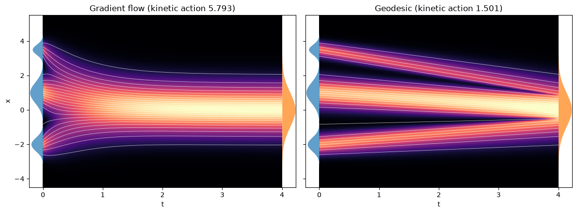
Back to the three levels
The Fokker-Planck section opened with three levels of description. Both paths of this section can now be placed on all three.
Once the principle is fixed, so is the density path: the gradient flow from has one solution, and so does the geodesic from to . The density path does not fix the particles, as the family of dynamics with shared marginals showed in the Fokker-Planck section. Diffusion and the geodesic differ in the principle, and that difference accounts for the factor of almost four between their actions.
Numerical checks
The JKO results depend on three numerical choices. Each one is varied separately, for the mixture with . The optimizer tolerance changes from to . The quantile grid doubles from to levels. The time step takes both values of , for both starting densities.References
- Benamou, J., Brenier, Y. (2000). A computational fluid mechanics solution to the Monge-Kantorovich mass transfer problem. Numer. Math. (Heidelb.). DOI
- Jordan, R., Kinderlehrer, D., Otto, F. (1998). The variational formulation of the Fokker—Planck equation. SIAM J. Math. Anal. DOI
- Santambrogio, F. (2015). Optimal transport for applied mathematicians – calculus of variations, PDEs and modeling.
Found an error on this page? Report an issue.