


Sampling and evaluating a density
The transport sections built maps and fields that turn samples of a simple source into samples of a target. A generative model often has a second job. Given a point , it should report how likely the model finds that point, the value of its density. You need this number to train by maximum likelihood, to compare models on held-out data, and to flag inputs the model finds unlikely. Sampling alone does not give you this number. If you push samples through a function , the outputs follow some density . To evaluate it at one point you have to know which produced and how much stretched the space around . A normalizing flow is a generative model built so that both are easy to compute: is invertible, and the stretch has a formula.The change of variables formula
Let have density on and let be an invertible, differentiable map of onto itself. The density of is where is the Jacobian matrix of the inverse map. The determinant measures how much scales a small volume around . Mass is conserved: the mass in a small cell around ends up in the image of that cell, so if spreads the cell over a larger volume, the density falls by the same factor. In 1D the Jacobian is the derivative, and the formula reads with . The transport maps and couplings section already built such a map. With , CDF , and the mixture CDF , the increasing map sends standard normal samples to samples of the mixture. It is the map of the transport sections, with in place of . It is increasing, so it is invertible, and it is a normalizing flow. The code below evaluates its change of variables density on a grid. It computes from the mixture CDF and the derivative by central differences. The result is the mixture density , with weights , means and standard deviations . The code also confirms that .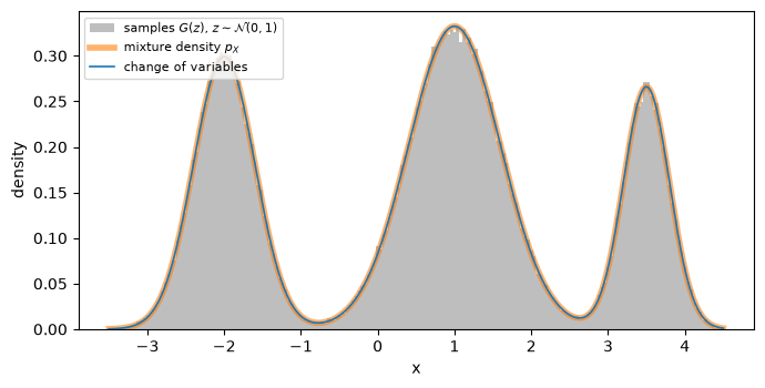
Composing maps
A single invertible layer is rarely flexible enough, so flows stack several. Write , start from , and set , so that . The determinant of a product of Jacobians is the product of their determinants, so the log-density picks up one term per layer: The terms add, so you can compute them layer by layer during the forward pass. The quantile map splits into two layers. The first, , sends to the uniform density on . The second, , sends the uniform density to the mixture. The code below computes each log-derivative by central differences at five points and adds the terms.Continuous flows
Stacking more and smaller layers leads to a flow in continuous time. A velocity field moves each particle by , and the map from to is invertible because you can run the same equation backward in time. The log-determinant of a stack becomes an integral along each trajectory. The integral follows from the continuity equation of the dynamic transport section, . Expanding the divergence of the product gives Along a trajectory the chain rule gives , which is the sum of the first two terms. So . Dividing by and integrating from to , This is the instantaneous change of variables formula of continuous normalizing flows (Chen et al., 2018). The divergence is the trace of the Jacobian of , so it replaces the determinant of the discrete formula. To evaluate at a point, integrate the trajectory backward from to find , and subtract the integral of the divergence along the way. The displacement interpolation of the dynamic transport section gives a check with a known answer. Each particle moves at the constant velocity , and in 1D the divergence is . The code below tracks 16,001 particles at evenly spaced quantile levels. At each time it estimates at every particle from the velocities and positions of its neighbors, and it integrates in time with the trapezoid rule. At the result matches the log of the mixture density at .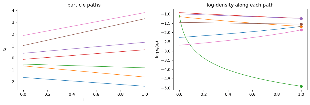
Flows, decoders and the models that follow
An invertible map keeps the dimension: and both live in . A latent-variable model such as the variational autoencoder decodes a low-dimensional into a high-dimensional . Its decoder has no inverse, so the density of is an integral over all that could have produced it, and training works with a lower bound on that integral. A flow has an exact density, but its latent space has as many dimensions as the data. The likelihood of a continuous flow is exact, but each evaluation integrates an ODE together with a divergence, and maximum likelihood training repeats that inside every gradient step. Flow matching trains the field of a continuous normalizing flow by regression on a chosen probability path (Lipman et al., 2022). It never evaluates a likelihood during training. After training, the formula above still gives the likelihood of any point under the learned field. The probability flow ODE of score-based diffusion is a deterministic flow with the same marginals as the diffusion, and the same integral of the divergence evaluates likelihoods for a diffusion model (Song et al., 2020). Key references: (Chen et al., 2018; Lipman et al., 2022; Song et al., 2020)References
- Chen, R., Rubanova, Y., Bettencourt, J., Duvenaud, D. (2018). Neural ordinary differential equations. arXiv [cs.LG]. DOI
- Lipman, Y., Chen, R., Ben-Hamu, H., Nickel, M., Le, M. (2022). Flow Matching for generative modeling. arXiv [cs.LG]. Link
- Song, Y., Sohl-Dickstein, J., Kingma, D., Kumar, A., Ermon, S., et al. (2020). Score-based generative modeling through stochastic differential equations. arXiv [cs.LG]. DOI
Found an error on this page? Report an issue.