Open In Colab

Particles, densities and principles

In the dynamic transport section every particle followed a velocity field, and its path was smooth. In the Brownian motion section particles moved at random, and the density still changed smoothly in time. This section asks whether deterministic dynamics can reproduce the densities of a random process. The answer needs three levels of description kept apart. This section works at the first two levels and ends with a measurement at the third: the kinetic action of the density path. The next section supplies the principle that diffusion follows.

The running example

The data distribution p0p_0 is the Gaussian mixture of the probability transport chapter, with weights πk=(0.3,0.5,0.2)\pi_k = (0.3, 0.5, 0.2), means μk=(−2,1,3.5)\mu_k = (-2, 1, 3.5) and standard deviations σk=(0.4,0.6,0.3)\sigma_k = (0.4, 0.6, 0.3). The forward process is the Ornstein-Uhlenbeck process of the Brownian motion section, dXt=−Xt dt+2 dWt,dX_t = -X_t\,dt + \sqrt{2}\,dW_t , so the drift is f(x)=−xf(x) = -x, the noise level is g=2g = \sqrt{2} and the diffusion coefficient is D=g2/2=1D = g^2/2 = 1. At each fixed tt, XtX_t has the same distribution as e−tX0+1−e−2t Ze^{-t} X_0 + \sqrt{1 - e^{-2t}}\,Z with Z∼N(0,1)Z \sim \mathcal{N}(0, 1) independent of X0X_0. The density ptp_t is therefore again a mixture of three Gaussians. Component kk keeps its weight, has mean μke−t\mu_k e^{-t} and has variance σk2e−2t+1−e−2t\sigma_k^2 e^{-2t} + 1 - e^{-2t}. This statement holds in distribution at each time separately, so paths below are built step by step, as in the drift part of the Brownian motion section. Because ptp_t is a mixture in closed form, so are its time derivative and its score ∂xlog⁡pt\partial_x \log p_t. The quantile function Ft−1F_t^{-1} comes from bisection on the closed-form CDF. Everything else on this page is numerical, and each place says how it was computed: particle paths come from integrator steps, distances between samples and densities from Monte Carlo, and actions from quadrature on a grid.

The horizon

The Ornstein-Uhlenbeck process reaches N(0,1)\mathcal{N}(0, 1) only as t→∞t \to \infty. Its distance to that limit shrinks at a known rate: W2(pt,N(0,1))≤e−t W2(p0,N(0,1)).W_2\bigl(p_t, \mathcal{N}(0, 1)\bigr) \le e^{-t}\, W_2\bigl(p_0, \mathcal{N}(0, 1)\bigr). The horizon TT is the smallest whole number at which this bound falls below 0.050.05. The bound and the computed distance at each whole tt up to TT follow.
The bound first drops below 0.050.05 at T=4T = 4, where the computed distance is smaller still. The endpoint pTp_T is close to N(0,1)\mathcal{N}(0, 1) but not equal to it, and this page always uses the true pTp_T.

Diffusion time and transport time

This page uses the diffusion convention: data at t=0t = 0 and noise at t=Tt = T. The probability transport chapter ran the other way, from noise at s=0s = 0 to data at s=1s = 1. The two clocks are related by s=1−t/T.s = 1 - t/T . The transport chapter’s p0p_0, the noise, is pTp_T here, and its p1p_1, the data, is p0p_0 here. Every figure on this page puts data on the left and noise on the right, so the transport chapter’s figures read in the opposite direction. The DDPM and DDIM sections use the variance-preserving SDE dX=−12β(t) X dt+β(t) dWdX = -\tfrac12 \beta(t)\,X\,dt + \sqrt{\beta(t)}\,dW. With the clock θ(t)=12∫0tβ(r) dr\theta(t) = \tfrac12 \int_0^t \beta(r)\,dr it becomes the Ornstein-Uhlenbeck process used here, so every result on this page carries over to those sections after a change of clock.

The Fokker-Planck equation

Conservation of mass gives an equation for ptp_t by the interval argument of the dynamic transport section. Let Jt(x)J_t(x) be the rate at which mass crosses xx from left to right. The mass in [a,b][a, b] changes only through the two ends, so ddt∫abpt dx=Jt(a)−Jt(b)=−∫ab∂xJt dx.\frac{d}{dt}\int_a^b p_t\,dx = J_t(a) - J_t(b) = -\int_a^b \partial_x J_t\,dx . This holds for every interval, so ∂tpt=−∂xJt\partial_t p_t = -\partial_x J_t at every point. Conservation alone says nothing about what JtJ_t is. The Brownian motion section supplied that: the drift carries mass with flux f pf\,p, and unbiased random steps carry mass down the gradient with the Fick flux −D ∂xp-D\,\partial_x p. Their sum gives the Fokker-Planck equation, ∂tpt=−∂x(f pt)+D ∂x2pt.\partial_t p_t = -\partial_x (f\,p_t) + D\,\partial_x^2 p_t . For the Ornstein-Uhlenbeck process it reads ∂tpt=∂x(x pt)+∂x2pt\partial_t p_t = \partial_x(x\,p_t) + \partial_x^2 p_t. The closed-form ptp_t should satisfy this equation. On the left, the analytic time derivative is taken through the moving means and variances of the components. On the right, the xx-derivatives are analytic too. The integrated residual ∫∣∂tpt−right side∣ dx\int |\partial_t p_t - \text{right side}|\,dx and the total mass ∫pt dx\int p_t\,dx are computed on [−12,12][-12, 12], at t=0.1,0.5,1,2t = 0.1, 0.5, 1, 2 and TT.
The residual is at the level of rounding error at every time, so the closed form of ptp_t solves the Fokker-Planck equation. The mass stays 1 to eight digits.

Drift, score and probability flow velocity

Pull ptp_t out of the total flux: Jt=f pt−D ∂xpt=pt (f−D ∂xlog⁡pt).\begin{aligned} J_t &= f\,p_t - D\,\partial_x p_t \\ &= p_t\,\bigl(f - D\,\partial_x \log p_t\bigr) . \end{aligned} The flux now has the form pt vtp_t\,v_t of the continuity equation, with the velocity vt(x)=f(x)−D ∂xlog⁡pt(x)=−x−∂xlog⁡pt(x).v_t(x) = f(x) - D\,\partial_x \log p_t(x) = -x - \partial_x \log p_t(x) . The Fokker-Planck equation is the continuity equation ∂tpt+∂x(pt vt)=0\partial_t p_t + \partial_x(p_t\,v_t) = 0 for this field. Particles that follow the ordinary differential equation x˙=vt(x)\dot x = v_t(x) from samples of p0p_0 therefore have density ptp_t at every time, the same as the particles of the SDE. This ODE is the probability flow ODE (Song et al., 2020). Three different quantities appear here. In deterministic transport the drift and the velocity are the same thing. With noise they differ by DD times the score. For a mixture, the score is a weighted sum of the component scores, with weights equal to the probability that xx came from each component. Computed this way it stays finite far in the tails, where ptp_t itself is too small to divide by. The same velocity has a second description. At each fixed time, XtX_t has the distribution of atX0+btZa_t X_0 + b_t Z with at=e−ta_t = e^{-t} and bt=1−e−2tb_t = \sqrt{1 - e^{-2t}}. A point on this interpolation moves with velocity a˙tX0+b˙tZ\dot a_t X_0 + \dot b_t Z. Average that velocity over all pairs (X0,Z)(X_0, Z) that pass through xx at time tt: ut(x)=E[a˙tX0+b˙tZ∣Xt=x].u_t(x) = \mathbb{E}\bigl[\dot a_t X_0 + \dot b_t Z \mid X_t = x\bigr] . Within one component, X0X_0, ZZ and XtX_t are jointly Gaussian, so the conditional means of X0X_0 and ZZ are linear in xx. Weighting them by the component probabilities gives ut(x)u_t(x) in closed form. Below, utu_t is compared with −x−∂xlog⁡pt-x - \partial_x \log p_t at t=0.1,0.5,1,2t = 0.1, 0.5, 1, 2 and TT, wherever pt>10−6p_t > 10^{-6}.
The two fields agree to rounding error. The probability flow velocity of this path is the conditional-mean field that flow matching regresses: the expected velocity a˙tX0+b˙tZ\dot a_t X_0 + \dot b_t Z of the interpolation Xt=atX0+btZX_t = a_t X_0 + b_t Z, given that it passes through xx. Flow matching and stochastic interpolants reach the same field from the interpolation, without the Fokker-Planck equation (Albergo et al., 2023).

Equilibrium

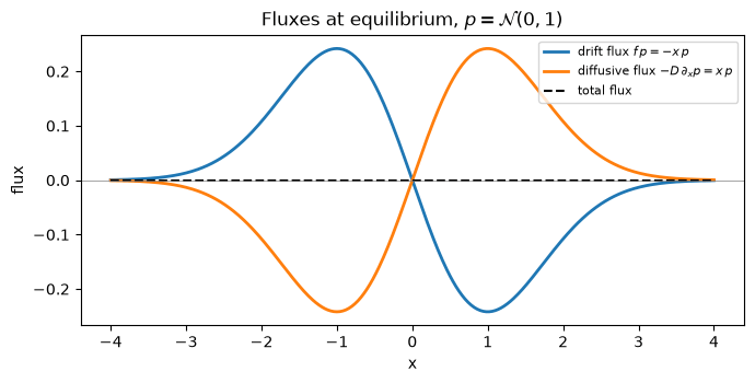
The simplest case shows the difference between drift and velocity. For p∞=N(0,1)p_\infty = \mathcal{N}(0, 1) the score is ∂xlog⁡p∞=−x\partial_x \log p_\infty = -x, so v∞(x)=−x−(−x)=0.v_\infty(x) = -x - (-x) = 0 . The density stands still while each particle keeps moving under dX=−X dt+2 dWdX = -X\,dt + \sqrt{2}\,dW. At every point the drift flux −x p∞-x\,p_\infty, which points toward the origin, cancels the diffusive flux −∂xp∞=x p∞-\partial_x p_\infty = x\,p_\infty, which points away from it. The rotation field of the velocity fields section is the deterministic analogue: there too the particles move while a rotationally symmetric density stays still. Two quantities confirm this: the general score function evaluated on N(0,1)\mathcal{N}(0, 1), and the velocity of the mixture path at t=40t = 40, where ptp_t equals N(0,1)\mathcal{N}(0, 1) to within e−40e^{-40}.
Line plot of three fluxes against x for the standard normal density. The drift flux, minus x times p, is positive for negative x and negative for positive x. The diffusive flux, x times p, is its mirror image. Their sum is a dashed line at zero everywhere. The two fluxes of N(0,1)\mathcal{N}(0, 1) and their sum. The drift pushes mass inward and diffusion spreads it outward at the same rate at every xx, so the total flux is zero and the density does not change.

Same marginals, different couplings

The SDE and the probability flow ODE are two members of a family. For every λ≥0\lambda \ge 0, dXt=[f+λ2−12 g2 ∂xlog⁡pt]dt+λ g dWt.\begin{aligned} dX_t &= \Bigl[f + \tfrac{\lambda^2 - 1}{2}\,g^2\,\partial_x \log p_t\Bigr] dt \\ &\quad + \lambda\,g\,dW_t . \end{aligned} Its drift flux is [f+(λ2−1)D ∂xlog⁡pt]pt\bigl[f + (\lambda^2 - 1) D\,\partial_x \log p_t\bigr] p_t and its diffusive flux is −λ2D ∂xpt-\lambda^2 D\,\partial_x p_t. Since pt ∂xlog⁡pt=∂xptp_t\,\partial_x \log p_t = \partial_x p_t, they add up to Jt=f pt−D ∂xptJ_t = f\,p_t - D\,\partial_x p_t for every λ\lambda. The flux is the same, so the Fokker-Planck equation is the same, and every member started from p0p_0 has the same density ptp_t at every time. The value λ=1\lambda = 1 gives the forward SDE and λ=0\lambda = 0 gives the probability flow ODE. The simulation starts 2000 samples of p0p_0 and moves the same samples under λ=0\lambda = 0, 0.50.5 and 11. For λ=1\lambda = 1 each step uses the exact Ornstein-Uhlenbeck transition. For the other two, each step is an Euler-Maruyama step of length 5×10−45 \times 10^{-4} with the exact score. If the marginals agree, the empirical W1W_1 distance from the particles to the closed-form ptp_t should be about as small as the W1W_1 distance of 2000 independent exact samples of ptp_t. That second distance, averaged over 20 draws, is the sampling baseline: the distance that sampling alone produces.
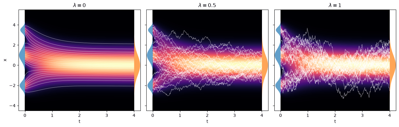
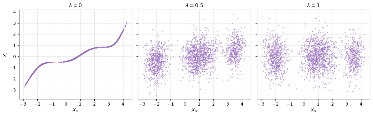
Three standard transport heatmaps for lambda equal to 0, 0.5 and 1, with time from 0 to 4 on the horizontal axis. The density is the same in all three: three bands at the left merge into one Gaussian band at the right. At lambda 0 the 25 white trajectories are smooth curves that never cross. At lambda 0.5 they are jagged and cross often. At lambda 1 they are rougher still and wander across the whole band. The same density path under three dynamics. Each panel shows ptp_t as a heatmap and 25 particle paths in white. At λ=0\lambda = 0 the paths are smooth and never cross. At λ=1\lambda = 1 they are Brownian. In all three panels the particles fill the same density. The densities agree, and the particles still end up in different places. A scatter of the starting point X0X_0 against the endpoint XTX_T shows the coupling that each dynamics produces. Three scatter plots of the final position against the starting position. For lambda 0 the points lie on one increasing curve with flat stretches between the three components. For lambda 0.5 and lambda 1 the points form three vertical clouds, one above each component, each spread over most of the range from -3 to 3. Starting point against endpoint for each λ\lambda. At λ=0\lambda = 0 the endpoint is an increasing function of the starting point. At λ=0.5\lambda = 0.5 the endpoint still depends on the starting point, but the coupling spreads widely. At λ=1\lambda = 1 the endpoint is nearly independent of X0X_0. All three dynamics have the same two marginals p0p_0 and pTp_T, and the couplings are different. The probability flow gives a deterministic, increasing map. The forward SDE gives a coupling close to independence, since four time units of noise have erased most of the starting position. This is the point of the maps and couplings section: the marginals do not fix the coupling. A later chapter on Schrödinger bridges picks one coupling among the stochastic ones by a principle of its own.

Running the flow backward

The probability flow ODE is deterministic, so it can be run from t=Tt = T back to t=0t = 0. Start from samples of pTp_T, integrate x˙=vt(x)\dot x = v_t(x) backward with 400 fourth-order Runge-Kutta steps, and the samples should arrive distributed as the mixture p0p_0. This is the deterministic sampler of diffusion models. A generative model starts from N(0,1)\mathcal{N}(0, 1) instead of pTp_T and learns the score instead of computing it; here both are exact, so only the integrator can introduce error. The DDIM section uses the same idea. Deterministic DDIM (η=0\eta = 0) is a discretization of the probability flow ODE of the variance-preserving SDE, in the clock θ\theta defined in the section on diffusion time.
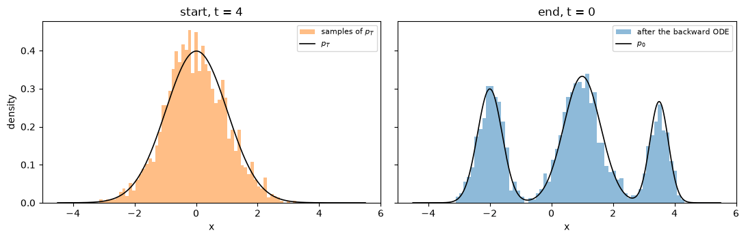
The recovered samples are within three times the sampling baseline of p0p_0. The integration error, measured below on the endpoint map, is about 10−610^{-6}. The remaining distance is consistent with the sampling noise of the 2000 starting points, carried through the map. Two histograms. On the left, 2000 samples of p_T follow the nearly Gaussian density p_T. On the right, the same samples after the backward flow follow the three-peaked mixture p_0, drawn as a black curve. Left, samples of pTp_T. Right, the same samples after the backward probability flow, with the mixture p0p_0 drawn in black.

Kinetic action of the density path

The dynamic transport section measured a path by its kinetic action. On this page the action belongs to the density path ptp_t and its velocity vtv_t. It does not belong to Brownian trajectories, which are nowhere differentiable. The discrete estimate E[(ΔX/Δt)2]\mathbb{E}\bigl[(\Delta X/\Delta t)^2\bigr] for the forward SDE grows like g2/Δtg^2/\Delta t, without limit as the step shrinks. One exact step of the forward SDE, started from samples of ptp_t at t=1t = 1, shows the growth.
Quartering the step quadruples the mean squared speed, close to g2/Δtg^2/\Delta t in both cases. The density path has a finite action. In physical time it is A=∫0T ⁣ ⁣∫pt(x) vt(x)2 dx dt.\mathcal{A} = \int_0^T \!\! \int p_t(x)\,v_t(x)^2\,dx\,dt . To compare it with the transport chapter, change to the normalized time s=1−t/Ts = 1 - t/T. The velocity becomes −T vt-T\,v_t, with the sign reversed because ss runs against tt, and ∣ds∣=dt/T|ds| = dt/T, so the action in normalized time is Aˉ=T A\bar{\mathcal{A}} = T\,\mathcal{A}. The Benamou-Brenier formula says that no path from p0p_0 to pTp_T has a smaller normalized action than W22(p0,pT)W_2^2(p_0, p_T) (Benamou & Brenier, 2000), so Aˉ≥W22\bar{\mathcal{A}} \ge W_2^2.

The endpoint map is the optimal map

The probability flow keeps particles in order, so its endpoint map is the increasing map FT−1∘F0F_T^{-1} \circ F_0. The 1D mixture section showed why an order-preserving flow ends at the optimal map on the line. Below, the flow is integrated forward from 99 quantile levels uu in [0.01,0.99][0.01, 0.99], the endpoints are compared with FT−1(u)F_T^{-1}(u), and the integration is repeated with half the step.
The flow reaches the optimal map to about 10−610^{-6}. It reaches it along a path that is not the geodesic, and the next part measures how much that path costs.

The excess, exactly

Write Qt=Ft−1Q_t = F_t^{-1} for the quantile function of ptp_t. The particle at level uu sits at Qt(u)Q_t(u), so ∂tQt(u)=vt(Qt(u))\partial_t Q_t(u) = v_t(Q_t(u)). The change of variable x=Qt(u)x = Q_t(u) turns pt dxp_t\,dx into dudu, and the action becomes A=∫0T ⁣ ⁣∫01∣∂tQt(u)∣2 du dt.\mathcal{A} = \int_0^T \!\! \int_0^1 \bigl|\partial_t Q_t(u)\bigr|^2\,du\,dt . The geodesic between p0p_0 and pTp_T moves every quantile at constant speed, Qtgeo=(1−t/T) Q0+(t/T) QTQ_t^{\text{geo}} = (1 - t/T)\,Q_0 + (t/T)\,Q_T, and W22=∫01∣QT−Q0∣2 duW_2^2 = \int_0^1 |Q_T - Q_0|^2\,du (Santambrogio, 2015). Expand the square below and use ∫0T∂tQt dt=QT−Q0\int_0^T \partial_t Q_t\,dt = Q_T - Q_0: Aˉ−W22=T∫0T ⁣ ⁣∫01∣∂tQt−QT−Q0T∣2du dt.\begin{aligned} \bar{\mathcal{A}} - W_2^2 &= T \int_0^T \!\! \int_0^1 \Bigl|\partial_t Q_t - \frac{Q_T - Q_0}{T}\Bigr|^2 du\,dt . \end{aligned} The excess action is the mean squared gap between the quantile speed and the constant geodesic speed. It is zero only when every quantile moves at constant speed. Numerically, Qt(u)Q_t(u) is evaluated on 1000 midpoint levels in [0.001,0.999][0.001, 0.999] and 801 times, spaced more densely near t=0t = 0, and ∂tQt\partial_t Q_t comes from central differences. The uu integrals cover [0.001,0.999][0.001, 0.999] only. Both Aˉ\bar{\mathcal{A}} and W22W_2^2 are truncated to the same range, so the inequality and the identity hold for the truncated quantities as well.
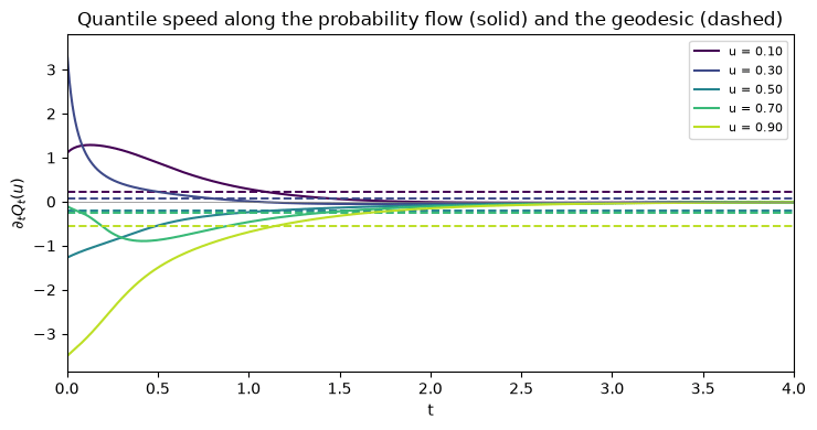
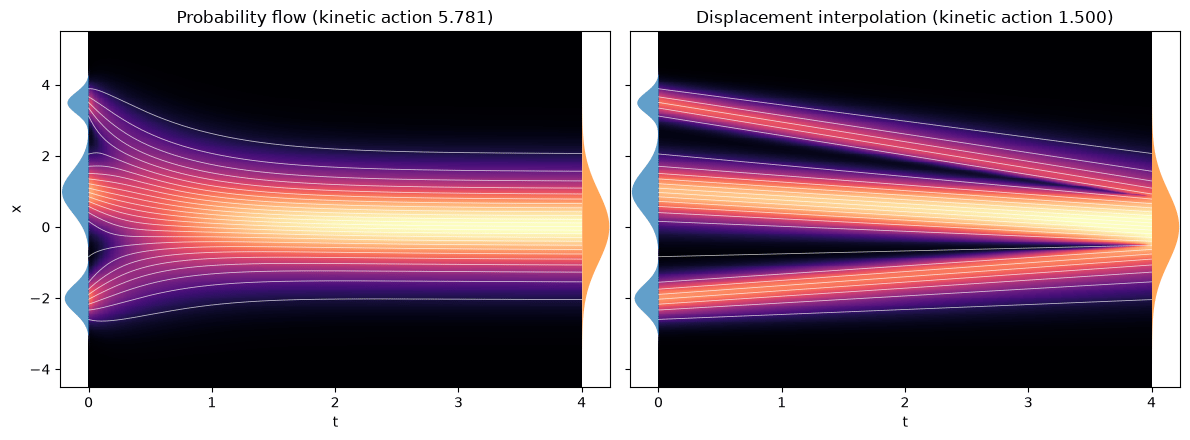
The probability flow has Aˉ=5.78\bar{\mathcal{A}} = 5.78, almost four times W22=1.50W_2^2 = 1.50. The quantile form of A\mathcal{A} agrees with the direct quadrature of ptvt2p_t v_t^2 over [Qt(0.001),Qt(0.999)][Q_t(0.001), Q_t(0.999)] with the exact velocity, and the two sides of the identity agree to four digits. The figure shows where the excess comes from. Quantile speed against time for five quantile levels from 0.1 to 0.9. Each solid curve starts far from zero at t = 0, as large as 3.5 in magnitude, and decays to nearly zero by t = 2. Each dashed horizontal line, the constant geodesic speed for the same level, stays between -0.6 and 0.3. Speed of five quantiles along the probability flow (solid) and along the geodesic (dashed, same color). The flow moves each quantile fast at the start and has almost stopped by t=2t = 2. The geodesic spreads the same displacement evenly over [0,T][0, T]. The quantiles move with the velocity vtv_t, and vtv_t follows the changes in ptp_t. The component means decay like e−te^{-t}, and the component variances change fastest near t=0t = 0, most of all for the narrow components. Both effects concentrate the motion near t=0t = 0. The squared speed penalizes an uneven schedule, as the h(t)=t2h(t) = t^2 schedule of the dynamic transport section did, so the front-loaded flow pays almost four times the geodesic cost for the same endpoint map. Two standard transport heatmaps with time from 0 to 4. On the left, the probability flow: the three bands of p_0 merge into one band before t = 1.5, and the quantile trajectories bend sharply at the start and are flat afterwards. Its title reports kinetic action 5.781. On the right, displacement interpolation: the trajectories are straight lines, the three bands stay apart until close to t = 4, and the title reports kinetic action 1.500. Left, the probability flow path with quantile trajectories at 25 levels. Right, displacement interpolation between p0p_0 and pTp_T, with straight trajectories. Both titles report the normalized action: Aˉ\bar{\mathcal{A}} on the left and W22W_2^2 on the right. The flow merges the three components before t=1.5t = 1.5. The geodesic keeps them apart until close to t=Tt = T.

From velocity to free energy

Diffusion does not take the geodesic, so the principle of least action does not explain the path it follows. The velocity vt=−x−∂xlog⁡ptv_t = -x - \partial_x \log p_t appears again in the next section, as the gradient of a free energy. That section shows that the Ornstein-Uhlenbeck path is the steepest descent of that free energy in the Wasserstein geometry.

Numerical checks

The checks below list the integrated Fokker-Planck residual and the mass at each check time, and the W1W_1 distances for the three values of λ\lambda beside their sampling baseline. They also compare the finite-difference quantile speed with the exact velocity vt(Qt)v_t(Q_t) away from t=0t = 0, and give the path-length split. With L(u)=∫0T∣∂tQt(u)∣ dtL(u) = \int_0^T |\partial_t Q_t(u)|\,dt the length of the path of quantile uu, the Cauchy-Schwarz inequality in tt and then the triangle inequality give Aˉ≥∫01L(u)2 du≥W22.\bar{\mathcal{A}} \ge \int_0^1 L(u)^2\,du \ge W_2^2 . The first gap is positive when a quantile moves at uneven speed. The second is positive when a quantile reverses direction along the way.
The residual, equilibrium and endpoint-map comparisons are repeated on a second mixture with weights (0.5,0.5)(0.5, 0.5), means (−1.5,2)(-1.5, 2) and standard deviations (0.5,0.5)(0.5, 0.5).

References

  • Albergo, M., Boffi, N., Vanden-Eijnden, E. (2023). Stochastic interpolants: A unifying framework for flows and diffusions. arXiv [cs.LG]. DOI
  • Benamou, J., Brenier, Y. (2000). A computational fluid mechanics solution to the Monge-Kantorovich mass transfer problem. Numer. Math. (Heidelb.). DOI
  • Santambrogio, F. (2015). Optimal transport for applied mathematicians – calculus of variations, PDEs and modeling.
  • Song, Y., Sohl-Dickstein, J., Kingma, D., Kumar, A., Ermon, S., et al. (2020). Score-based generative modeling through stochastic differential equations. arXiv [cs.LG]. DOI

Found an error on this page? Report an issue.