Markov Random Fields and Belief Propagation

This section was written by Kaushik Kachireddy (pull request #81), with help from an AI coding agent (Claude Code) on the code. It reproduces the ideas of Chapter 29 of Foundations of Computer Vision by Antonio Torralba, Phillip Isola, and William T. Freeman. The book’s own figures are not reproduced here, because the book’s license covers only the work in full; links point to them instead. A graphical model factorizes a joint distribution over many variables into a product of local terms tied to the edges of a graph. For vision the variables are per-pixel labels (a depth, a segment, a clean intensity), and the graph encodes which labels should agree. This section builds:

The MRF smoothness prior, sampled with Gibbs sampling.
Exact belief propagation on a tree, reproducing the book’s numerical example (Figure 29.15) and checking it against brute-force marginalization.
Loopy belief propagation on the image grid, for binary denoising.
Segmentation of a photograph by loopy BP (the book’s version is Figure 29.4).
Stereo along one scanline of a real stereo pair by BP (Figure 29.14), checked against ground truth.

The book uses its own photographs, a leaf and a canoe stereo pair. Here the same algorithms run on scikit-image’s coins image and on the Middlebury motorcycle stereo pair, which comes with ground-truth disparity.

import numpy as np
import matplotlib.pyplot as plt
from skimage.transform import resize

rng = np.random.default_rng(0)
plt.rcParams.update({'figure.dpi': 130, 'savefig.dpi': 130,
                     'image.cmap': 'gray', 'image.interpolation': 'nearest', 'axes.grid': False})

from skimage import data, img_as_float
# stand-in for a photograph of a leaf in the book; original: https://visionbook.mit.edu/figures/graphical_models/leaf1.jpg
COINS = img_as_float(data.coins())                  # image to be segmented (in place of the book's leaf, 29.4)
# stand-in for a stereo pair of canoes in the book; original: https://visionbook.mit.edu/graphical_models.html#fig-canoe1
MOTO_L, MOTO_R, MOTO_DISP = data.stereo_motorcycle()  # rectified Middlebury pair + ground-truth disparity (29.14)
MOTO_L, MOTO_R = img_as_float(MOTO_L), img_as_float(MOTO_R)
print('coins', COINS.shape, ' motorcycle', MOTO_L.shape)

coins (303, 384)  motorcycle (500, 741, 3)

Images replaced for licensing. The book is published under a CC BY-NC-ND license, which covers only the book as a whole and not its individual images, so this page does not republish the book’s photographs. License-free images stand in for them:

The coins image (scikit-image) stands in for a photograph of a leaf (Figure 29.4).
The Middlebury motorcycle stereo pair (scikit-image) stands in for a stereo pair of canoes (Figures 29.12 to 29.14).

If you use the book for non-commercial purposes, you can swap the originals back in: each line that loads a stand-in carries the original’s link in a comment.

The MRF prior: neighboring pixels agree

An undirected graphical model (Markov random field) puts a potential on every edge. The workhorse prior for images is the Ising / Potts model, which rewards neighboring pixels for taking the same label:

p(\mathbf{x}) \propto \exp\Big(\beta \textstyle\sum_{(i,j)\in\mathcal{E}} \mathbb{1}[x_i = x_j]\Big).

There is no data here: this is purely the prior. To see what it believes, draw samples with Gibbs sampling: repeatedly replace each pixel by a draw from its conditional given its four neighbors. Because the grid is bipartite, all black-square pixels are conditionally independent given the white-square ones, so a whole color can be updated at once (checkerboard sweeps). As the coupling

\beta

grows, samples go from white noise to ever-larger smooth regions: exactly the ‘images are piecewise smooth’ assumption the rest of the chapter exploits.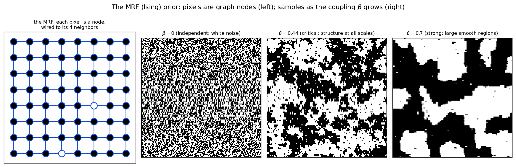

def ising_gibbs(size, beta, sweeps=40, seed=0):
    g = np.random.default_rng(seed)
    x = g.integers(0, 2, size=(size, size)) * 2 - 1          # spins in {-1,+1}
    i, j = np.indices((size, size))
    for _ in range(sweeps):
        for color in (0, 1):                                # checkerboard: update one color
            nb = np.zeros_like(x, float)                     # sum of 4 neighbors
            nb[1:] += x[:-1]; nb[:-1] += x[1:]
            nb[:, 1:] += x[:, :-1]; nb[:, :-1] += x[:, 1:]
            p_up = 1.0 / (1.0 + np.exp(-2.0 * beta * nb))     # P(x_i = +1 | neighbors)
            flip = (g.random((size, size)) < p_up) * 2 - 1
            x = np.where((i + j) % 2 == color, flip, x)
    return x

Exact belief propagation on a tree

On a graph without loops, belief propagation computes the exact marginals. This part reproduces the book’s worked example (Fig 29.15): a chain

x_1 - x_2 - x_3

with an observed node

y_2 = 0

hanging off

x_2

. Every variable is binary and the potentials are exactly those printed in the figure:

\psi_{12}=\begin{pmatrix}1.0&0.9\\0.9&1.0\end{pmatrix},\quad\psi_{23}=\begin{pmatrix}0.1&1.0\\1.0&0.1\end{pmatrix},\quad\phi_{2}=\begin{pmatrix}1.0&0.1\\0.1&1.0\end{pmatrix}.

Sum-product rule: a node collects the incoming messages, and the message it sends across an edge is

m_{a\to b}(x_b)=\sum_{x_a}\psi_{ab}(x_a,x_b)\,\phi_a(x_a)\prod_{c\ne b}m_{c\to a}(x_a)

. A node’s marginal is the (normalized) product of all its incoming messages times its own evidence. Because this graph is a tree, BP must agree with brute-force marginalization over all

2^3

joint states: the code checks that it does.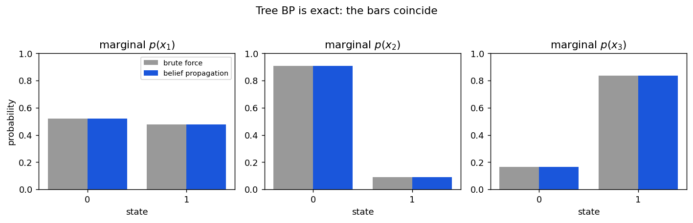

psi12 = np.array([[1.0, 0.9], [0.9, 1.0]])
psi23 = np.array([[0.1, 1.0], [1.0, 0.1]])
phi2  = np.array([[1.0, 0.1], [0.1, 1.0]])
ev2 = phi2[:, 0]                     # evidence on x2 from the observation y2 = 0  -> [1.0, 0.1]
norm = lambda v: v / v.sum()

# --- Sum-product BP on the tree (leaves -> x2 -> leaves) ---
m_1to2 = psi12.T @ np.ones(2)        # leaf x1 sends: sum_{x1} psi12(x1,x2)
m_3to2 = psi23   @ np.ones(2)        # leaf x3 sends: sum_{x3} psi23(x2,x3)
bel2 = norm(ev2 * m_1to2 * m_3to2)
m_2to1 = psi12 @ (ev2 * m_3to2)      # x2 -> x1 (fold in evidence and the x3 branch)
m_2to3 = psi23.T @ (ev2 * m_1to2)    # x2 -> x3
bel1, bel3 = norm(m_2to1), norm(m_2to3)
bp = np.array([bel1, bel2, bel3])

# --- Brute force: full joint over (x1,x2,x3) ---
brute = np.zeros((3, 2))
Z = 0.0
for a in (0, 1):
    for b in (0, 1):
        for c in (0, 1):
            w = psi12[a, b] * psi23[b, c] * ev2[b]
            Z += w
            brute[0, a] += w; brute[1, b] += w; brute[2, c] += w
brute /= Z

print('node   P(x=0)  P(x=1)      BP == brute force?')
for k in range(3):
    print(f'  x{k+1}   {bp[k,0]:.4f}  {bp[k,1]:.4f}    '
          f'{np.allclose(bp[k], brute[k])}')
assert np.allclose(bp, brute)

node   P(x=0)  P(x=1)      BP == brute force?
  x1   0.5215  0.4785    True
  x2   0.9091  0.0909    True
  x3   0.1653  0.8347    True

Loopy belief propagation on the image grid

The image grid has loops, so BP is no longer exact: but loopy BP (just keep passing messages) works remarkably well in practice. For binary labels every message is a two-vector, which the code track by its log-odds

m = \log\frac{m(1)}{m(0)}

. Passing a log-odds belief

b

through an Ising edge with coupling

J

gives the closed form

m_{\text{out}} = \log\frac{e^{J}e^{b}+e^{-J}}{e^{-J}e^{b}+e^{J}},

which is applied to all edges of one orientation at once with array shifts. The first test is denoising: a clean binary image is corrupted by flipping 20% of the pixels; the per-pixel likelihood gives each node a data log-odds

\pm\log\frac{1-q}{q}

, and the Ising prior glues neighbors together.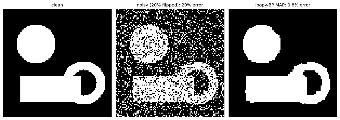

def ising_edge(b_in, J):
    '''Outgoing log-odds along one Ising edge given incoming node log-odds b_in.'''
    return np.logaddexp(J + b_in, -J) - np.logaddexp(-J + b_in, J)

def loopy_bp_binary(data_logodds, J, iters=30):
    '''Loopy BP on a 4-connected grid of binary nodes; returns posterior log-odds.'''
    mU = np.zeros_like(data_logodds); mD = np.zeros_like(data_logodds)
    mL = np.zeros_like(data_logodds); mR = np.zeros_like(data_logodds)
    for _ in range(iters):
        b = data_logodds + mU + mD + mL + mR              # current node beliefs
        oR = ising_edge(b - mR, J); nL = np.zeros_like(mL); nL[:, 1:] = oR[:, :-1]
        oL = ising_edge(b - mL, J); nR = np.zeros_like(mR); nR[:, :-1] = oL[:, 1:]
        oD = ising_edge(b - mD, J); nU = np.zeros_like(mU); nU[1:, :] = oD[:-1, :]
        oU = ising_edge(b - mU, J); nD = np.zeros_like(mD); nD[:-1, :] = oU[1:, :]
        mL, mR, mU, mD = nL, nR, nU, nD
    return data_logodds + mU + mD + mL + mR

# clean binary image: disk, bar, ring
yy, xx = np.mgrid[0:100, 0:100]
clean = np.zeros((100, 100), int)
clean[(yy - 32) ** 2 + (xx - 30) ** 2 < 18 ** 2] = 1
clean[62:86, 16:72] = 1
ring = (yy - 68) ** 2 + (xx - 74) ** 2
clean[(ring < 20 ** 2) & (ring > 12 ** 2)] = 1

q = 0.20                                              # pixel flip probability
flips = np.random.default_rng(1).random(clean.shape) < q
noisy = np.where(flips, 1 - clean, clean)
L = np.log((1 - q) / q)
data_lo = (2 * noisy - 1) * L                        # data log-odds favoring label 1
post = loopy_bp_binary(data_lo, J=1.0, iters=40)
denoised = (post > 0).astype(int)

err_noisy = (noisy != clean).mean(); err_bp = (denoised != clean).mean()

print(f'pixel error  {err_noisy:.1%}  ->  {err_bp:.1%}   after loopy BP')

pixel error  20.0%  ->  0.8%   after loopy BP

Segmentation as a two-label MRF

The same machinery segments a photograph: label each pixel object or background. The book segments a leaf by its color; here the evidence is brightness, on an image of coins against a darker background. The local evidence is how much brighter each pixel is than the median, turned into log-odds. On its own it gives a ragged, speckled mask; the smoothness prior cleans it into solid regions with short boundaries.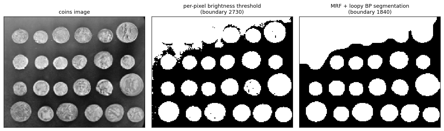

img = resize(COINS, (150, round(150 * COINS.shape[1] / COINS.shape[0])), anti_aliasing=True)
data_lo = 2.0 * (img - np.median(img)) / (img.std() + 1e-9)   # brighter than typical -> 'object'
raw = data_lo > 0                                    # per-pixel threshold (no prior)
seg = loopy_bp_binary(data_lo, J=1.0, iters=30) > 0  # with the smoothness prior

boundary = lambda m: int(np.abs(np.diff(m.astype(int), axis=0)).sum()
                         + np.abs(np.diff(m.astype(int), axis=1)).sum())

Stereo along a scanline

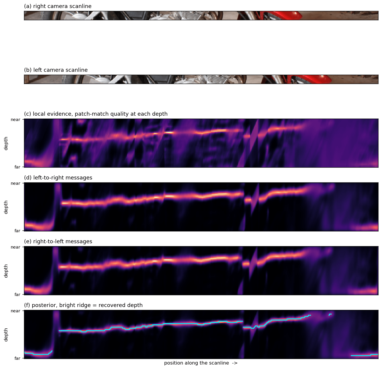
Stereo makes the graphical-model picture concrete (Fig 29.14). Take one scanline from the rectified left and right views of a rectified stereo pair (the book uses a canoe; here, the Middlebury motorcycle). Each pixel position is a node whose label is a disparity (depth); the local evidence is how well the left patch matches the right patch shifted by that disparity, and the chain of nodes is tied by a smoothness prior. The code runs sum-product BP along the 1-D chain: a forward (left-to-right) sweep and a backward (right-to-left) sweep, then multiply them with the evidence to get the marginal posterior at every position. How to read the panels below (they mirror the book):

(a), (b) the same row of pixels seen by the right and left cameras.
(c) to (f) are position × depth images: the horizontal axis is position along the scanline (lined up with a,b) and the vertical axis is candidate depth (small disparity = far, large = near). Brighter = more probable. So each vertical slice is a probability-over-depth for one pixel.
(c) local evidence: how well the left patch matches the right patch at each depth. Textured regions give a sharp bright spot (confident); smooth surfaces are ambiguous (diffuse).
(d), (e) messages: belief passed left→right and right→left along the chain, carrying confident estimates into the ambiguous regions.
(f) posterior = evidence × both messages. The bright ridge is the recovered depth profile; it is overlaid as a line.

It is a deliberately simple matcher (windowed normalized correlation + a truncated-linear smoothness), so it captures the behavior of Fig 29.14 rather than the book’s exact pixels. Because this pair has ground-truth disparity, the code also measures the error.

# --- extract one scanline band from each view; the pair is rectified, so it is the same row ---
row, band, win = 300, 8, 7
SL = MOTO_L[row - band:row + band + 1]           # (2*band+1, W, 3)
SR = MOTO_R[row - band:row + band + 1]
W = MOTO_L.shape[1]
gt_row = MOTO_DISP[row]                          # ground-truth disparity along the scanline
lo, hi = np.percentile(gt_row[np.isfinite(gt_row)], [2, 98])
G, DELTA = int(round((lo + hi) / 2)), int(np.ceil((hi - lo) / 2)) + 2   # center and half-width of the search
disps = np.arange(G - DELTA, G + DELTA + 1); D = len(disps)

def zwin(S, x):                                  # zero-mean unit-norm patch (for NCC)
    v = S[:, x - win:x + win + 1].ravel(); v = v - v.mean()
    return v / (np.sqrt((v * v).sum()) + 1e-9)

# local evidence phi[x, d] from 1 - normalized cross-correlation
cost = np.ones((W, D))
for x in range(win + G, W - win):
    a = zwin(SL, x)
    for j, d in enumerate(disps):
        xr = x - d
        if win <= xr < W - win:
            cost[x, j] = 1.0 - a @ zwin(SR, xr)
phi = np.exp(-cost / 0.25); phi /= phi.sum(1, keepdims=True)

# truncated-linear smoothness: cheap to disagree a little, capped so depth edges survive
dd = np.abs(disps[:, None] - disps[None, :])
psi = np.exp(-np.minimum(dd, 4) / 1.2)

def nrm(v): s = v.sum(); return v / s if s > 0 else np.full_like(v, 1.0 / len(v))
mfwd = np.ones((W, D)) / D                        # left-to-right messages
for x in range(1, W): mfwd[x] = nrm(psi.T @ (phi[x - 1] * mfwd[x - 1]))
mbwd = np.ones((W, D)) / D                        # right-to-left messages
for x in range(W - 2, -1, -1): mbwd[x] = nrm(psi @ (phi[x + 1] * mbwd[x + 1]))
posterior = phi * mfwd * mbwd; posterior /= posterior.sum(1, keepdims=True)

vis = slice(G + win, W - win)                     # valid (matchable) columns only
post_idx = posterior[vis].argmax(1)               # recovered depth profile (MAP)
panels = [(phi, '(c) local evidence, patch-match quality at each depth'),
          (mfwd, '(d) left-to-right messages'),
          (mbwd, '(e) right-to-left messages'),
          (posterior, '(f) posterior, bright ridge = recovered depth')]

jit = lambda m: np.abs(np.diff(disps[m[vis].argmax(1)])).mean()
print(f'disparity jitter along the scanline:  winner-take-all {jit(phi):.2f}  ->  BP {jit(posterior):.2f}')
gt_vis = gt_row[vis]; ok = np.isfinite(gt_vis)
err = lambda m: np.abs(disps[m[vis].argmax(1)] - gt_vis)[ok].mean()
print(f'mean |disparity error| vs ground truth:  winner-take-all {err(phi):.2f} px  ->  BP {err(posterior):.2f} px')

disparity jitter along the scanline:  winner-take-all 0.31  ->  BP 0.20
mean |disparity error| vs ground truth:  winner-take-all 3.37 px  ->  BP 3.37 px

Belief propagation makes the recovered profile smoother and carries confident depths across the ambiguous stretches, which shows as the lower jitter. The mean error against ground truth barely moves, because it is dominated by the textureless floor at the right end of the scanline: there, neither method has any evidence to work with, and a single chain of pixels cannot borrow it from neighboring rows. Full stereo methods run inference over the whole image grid for that reason.

Summary

A graphical model splits an image problem into local evidence (data terms) and a smoothness prior (edge potentials); inference combines them.
On a tree, sum-product BP is exact: it matched brute force to machine precision (29.15). On the looped image grid, loopy BP is approximate but effective for denoising, segmentation, and stereo.
BP is message passing: each node’s belief is the product of its neighbors’ messages and its own evidence. Smoothness lets confident, textured regions propagate into ambiguous, textureless ones.
These MRF and BP energies are the classical ancestors of today’s dense-prediction networks. The priors are now learned, but the evidence-plus-smoothness structure remains.

Edit this page on GitHub or file an issue.

Perception

Image Processing

CNNs

Scene Understanding

Faster RCNN Lab

YOLO Lab

UNet Lab

Mask RCNN Lab

Markov Random Fields and Belief Propagation

The MRF prior: neighboring pixels agree

Exact belief propagation on a tree

Loopy belief propagation on the image grid

Segmentation as a two-label MRF

Stereo along a scanline

Summary

​The MRF prior: neighboring pixels agree

​Exact belief propagation on a tree

​Loopy belief propagation on the image grid

​Segmentation as a two-label MRF

​Stereo along a scanline

​Summary

The MRF prior: neighboring pixels agree

Exact belief propagation on a tree

Loopy belief propagation on the image grid

Segmentation as a two-label MRF

Stereo along a scanline

Summary