Region Proposals
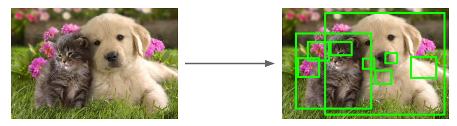
We can think about the detection problem as a classification problem of all possible portions (windows/masks) of the input image since an object can be located at any position and scale in the image. It is natural to search therefore everywhere and an obvious method to generate region proposals, is to slide various width-height ratio windows around the image and using a metric to declare that the window contains one or more blob of pixels. Such method is computationally infeasible and we need to think of how to reduce this number by employing an algorithm to guide where to look in the image for possible general object instances. Such algorithm is called selective search via hierarchical grouping and is used by the baseline RCNN implementation, noting that the RCNN detector can accommodate a number of other algorithms for such purpose.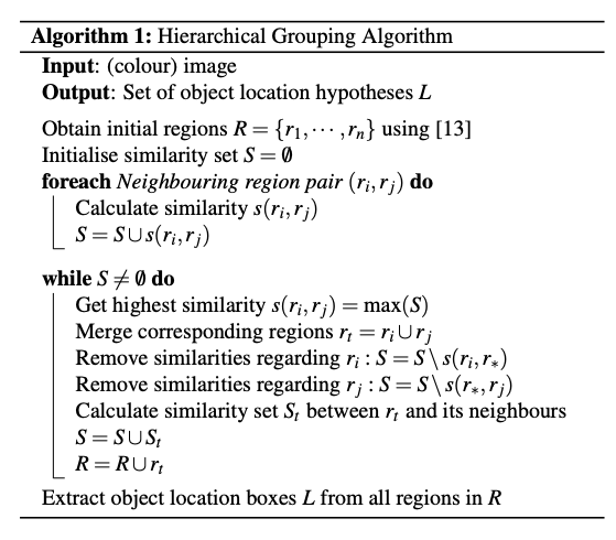
Graph-based segmentation
The hierarchical grouping algorithm itself uses a graph-based segmentation scheme to obtain the set of initial regions. The segmentation algorithm starts by formulating the image as a graph. Let G = (V, E) be an undirected graph with vertices , the set of elements to be segmented, and edges corresponding to pairs of neighboring vertices. Each edge has a corresponding weight , which is a non-negative measure of the dissimilarity between neighboring elements and . In the case of image segmentation, the elements in are pixels and the weight of an edge is some measure of the dissimilarity between the two pixels connected by that edge (e.g., the difference in intensity, color, motion, location or some other local attribute). A segmentation is a partition of into components such that each component (or region) corresponds to a connected component in a graph , where . In other words, any segmentation is a subset of the edges in . There are different ways to measure the quality of a segmentation but in general we want the elements in a component to be similar, and elements in different components to be dissimilar. This means that edges between two vertices in the same component should have relatively low weights, and edges between vertices in different components should have higher weights. For example, a pixel corresponds to a vertex and it has 8 neighboring pixels. We can define the weight to be the absolute value of the dissimilarity between the pixel light intensity and its neighbors. Before we compute the weights we use the 2D Gaussian kernel / filter we met in the earlier discussion on CNN filters - the end result being a smoothing of the image that helps with noise reduction. For color images we run the algorithm for each of the three channels. There is one runtime parameter for the algorithm, which is the value of that is used in the threshold function where is the number of elements in the sect . Thus a larger causes a preference for larger components. The graph algorithm can also accommodate dissimilarity weights between neighbors at a feature space rather at pixel level based on a Euclidean distance metric with other distance functions possible.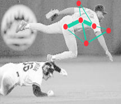
Grouping
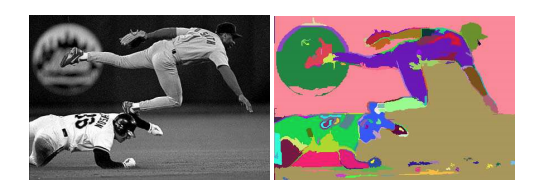
After the initial regions are produced, we use a greedy algorithm to iteratively group regions together. This is what gives the hierarchical in the name of the algorithm. First the similarities between all neighboring regions are calculated. The two most similar regions are grouped together, and new similarities are calculated between the resulting region and its neighbors. The process of grouping the most similar regions is repeated until the whole image becomes a single region. For the similarity between region and we apply a variety of complementary measures under the constraint that they are fast to compute. In effect, this means that the similarities should be based on features that can be propagated through the hierarchy, i.e. when merging region and into , the features of region need to be calculated from the features of and without accessing the image pixels. Such feature similarities include color, texture, size, fill - we create a binary sum of such individual similarities. where denotes if the similarity measure is used or not. The end result of the grouping is a hierarchy of regions ranked according to creation time. As earlier created regions may end up being the largest some permutation in the ranking is applied.
Training the RCNN
Each of these proposals is then fed into a CNN - since regions are of various rectangular shapes, we warp the regions to a fixed size since CNNs can only process fixed input tensors. The CNN used at the time was AlexNet that required pixels. The original AlexNet was pretrained on ImageNet and the weights were frozen. The ImageNet dataset has 1000 classes and as a result the last layer of the CNN classifier is a softmax layer that produces a 1000-dim vector. We need to start from this network and finetune for the task and domain at hand.Finetuning over all classes
To start, we replace the pretrained network head with a new head that matches the number of classes we are interested in. For example for the COCO dataset the number of classes is 80 plus the background class. We then continue from the pretrained weights and finetune the network on the new dataset that consists of warped region images and region labels - the later are assigned as follows: We have the ground truth bounding boxes for the original training images. and not for the region proposals and therefore we form a new finetuning classification dataset where,- all proposals that have with the ground truth box that belongs to the class are declared as positive proposals for this class assigning these proposals the label and
- the rest are treated as negative (background) assigning these proposals the, typical for background, label 0.
Note the important difference between this arrangement and typical classification tasks. Here, because of the introduction of the background class in the classification head, we are able to easily produce an objectness score which is assuming that 0 is the index of the background class. We could use the output directly to classify the region as being in class or not, but the IoU filtering we did earlier underrepresents hard negatives (negatives that have and therefore are borderline cases) and we will pay a performance penalty. We address this in the next section.
Binary classification per class
After finetuning, the CNN can produce a 4096-dim feature vector from each of the regions. Note that this representation of each region is shared across classes, in other words the feature vector does not represent a class but the “object-ness” of each region. We attach a binary Support Vector Machine (SVM) linear classifier head to the CNN portion of the network, swapping the K+1 classification head we had in the finetuning stage. Using these stored features the binary classifier produces a positive or negative prediction on whether this feature contains the class of interest or not. We train a separate binary SVM classifier per class, using a binary classification dataset that is itself produced from the original training dataset using yet another time the IoU and a new threshold . We label as positive examples only the ground truth boxes of the corresponding class and therefore assign them the label 1. Negative example are all the regions that have IoU with the ground truth box less than and therefore are assigned the label 0. We ignore the rest of the regions that have and are not ground truth boxes.Linear Regression for bounding box adjustment
Finally, a bounding box regressor, predicts the location of the bounding boxes using the proposal boxes and nearby ground truth box data so that we can adjust the final detection box and avoid situations that whole objects are detected but partially included in the detection box. The details of the bounding box regressor are shown in Annex C of the original paper and since this regression is going to be replaced by more modern methods we will not go into details here.Inference
Inference is made by feeding through the CNN the region proposals and then scoring each region with the SVM classifier.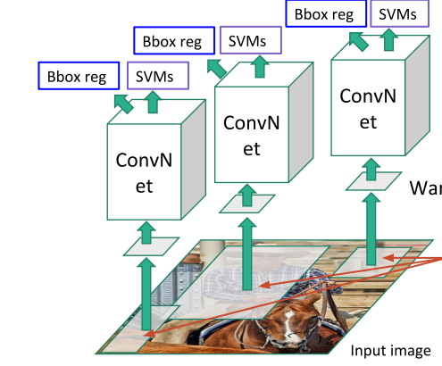
Non-Max Suppression (NMS)
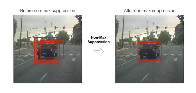
After the scoring of each proposed region by the SVM we apply a greedy Non-Maximum Suppression (NMS) algorithm for each class independently, that rejects a region if it has an Intersection over Union (IoU) metric with a higher scoring region, higher than a threshold . This threshold was empirically determined to be for the task outlined in the paper, but it is expected to be a hyperparameter in practice. The NMS algorithm is shown below: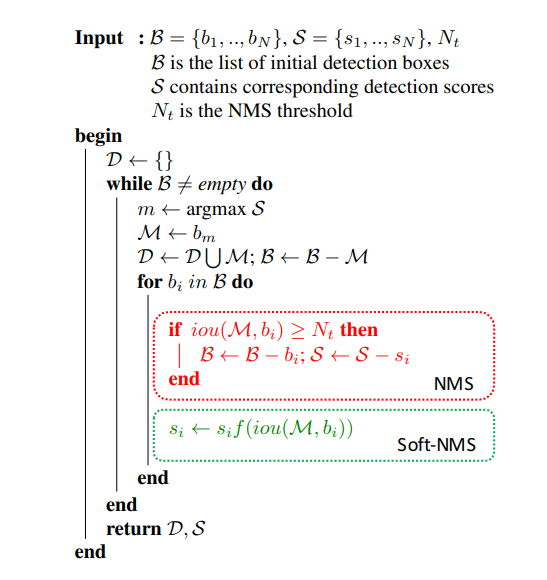
An issue with non-maximum suppression is that it sets the score for neighboring detections to zero. Thus, if an object was actually present in that overlap threshold, it would be missed and this would lead to a drop in average precision. However, if we lower the detection scores as a function of its overlap with M , it would still be in the ranked list, although with a lower confidence.
PyTorch reference
| PyTorch class | Description |
|---|---|
nn.Conv2d | Applies a 2D convolution over an input signal composed of several input planes. |
nn.ReLU | Applies the rectified linear unit function element-wise. |
nn.MaxPool2d | Applies a 2D max pooling over an input signal composed of several input planes. |
nn.Linear | Applies an affine linear transformation to the incoming data: . |
References
- Liu, W., Anguelov, D., Erhan, D., Szegedy, C., Reed, S., et al. (2015). SSD: Single Shot MultiBox Detector.
- Redmon, J., Divvala, S., Girshick, R., Farhadi, A. (2015). You only look once: Unified, real-time object detection.
- Ren, S., He, K., Girshick, R., Sun, J. (2015). Faster R-CNN: Towards Real-Time Object Detection with Region Proposal Networks.
- Sermanet, P., Eigen, D., Zhang, X., Mathieu, M., Fergus, R., et al. (2013). OverFeat: Integrated Recognition, Localization and Detection using Convolutional Networks.
- Shrivastava, A., Gupta, A., Girshick, R. (2016). Training Region-based Object Detectors with Online Hard Example Mining.