Introduction to Convolutional Neural Networks

​

Vision as a hierarchy of features

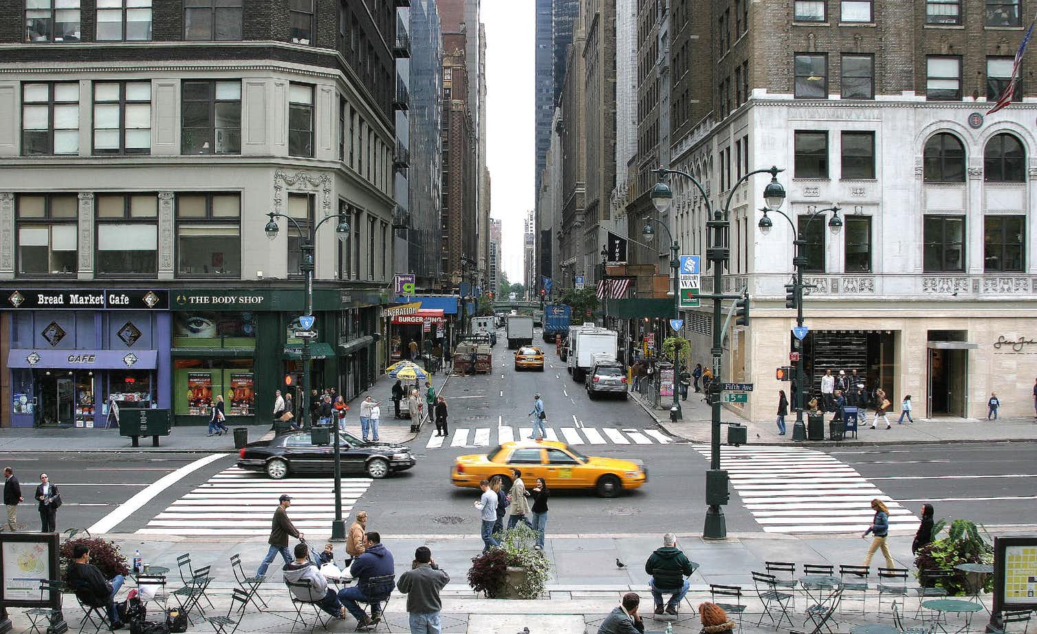
Most people notice the yellow cab first. When you look at this image, you take in the whole scene at a glance, a city street, before you settle on any one object, here most likely the yellow cab. Your brain builds a schematic representation of the scene across eye fixations, called the scene gist (how the brain reconstructs the visual world). The gist holds the scene’s basic category (natural, human-made, urban) and its general layout, and only a few objects or features. It is far from a detailed picture in the head. It guides each next fixation, which then samples more detail. The detail starts from simple, local measurements. David Hubel and Torsten Wiesel found that many neurons in the primary visual cortex, V1, at the back of the brain, respond to an edge of a particular orientation within a small patch of the visual field (simple cells), and that other neurons respond to the same oriented edge anywhere within a larger region, as if pooling several simple cells (complex cells). This hierarchy of local detectors followed by pooling inspired Fukushima’s neocognitron (1980), an early ancestor of the convolutional neural network. A CNN builds the same kind of hierarchy: its first layers learn small oriented filters, and deeper layers combine them into detectors of parts and objects. The operation that applies one filter at every position of an image is convolution.

​

The Convolution & Cross-Correlation Operation

The key operation performed in CNN layers is that of 2D convolution. In fact in practice they are 4D convolutions as we try to learn many filters and we also consider many input images (mini-batch) in the iteration of our SGD optimizer. Convolution itself, in one and two dimensions, with its properties and boundary handling, is covered in Convolution and Linear Filters. Here you need only the 2D case and how a CNN layer uses it.

​

2D Convolution

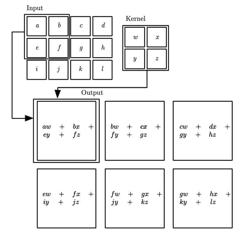
The 2D convolution of an input $x$ with a kernel (filter) $h$, usually much smaller than the input, is $S(i,j) = \sum_m \sum_n x(m, n) h(i-m,j-n) = \sum_m \sum_n x(i-m, j-n)h(m,n)$ Convolution is commutative, so you can flip either the input or the kernel; frameworks differ only in which form they write. Many ML frameworks don’t even implement convolution: they compute the very similar cross-correlation and call it convolution, which adds to the confusion. Both PyTorch’s Conv2d and TensorFlow compute cross-correlation under the hood: $S(i,j) = \sum_u \sum_v x(i+u, j+v)h(u,v)$ Cross-correlation, as a CNN layer computes it: the kernel slides over the input without being flipped, and each output is the weighted sum of the input window under it. Keeping only positions where the kernel lies entirely inside the input (“valid” convolution), a $3 \times 4$ input and a $2 \times 2$ kernel give a $2 \times 3$ output feature map. Figure 9.1 of Goodfellow, Bengio and Courville, Deep Learning (MIT Press, 2016). Whether the network learns the kernel or its flipped version makes no difference to the task of predicting the right label, because the flip is absorbed into the learned weights. What matters is the operation itself: a small set of weights applied at every position of the input.

​

From fixed filters to learned filters

Classical image processing applies filters whose weights you choose by hand: a box or Gaussian kernel to blur an image (Smoothing an Image with Blur Filters), or a derivative kernel to find edges (Measuring Change with Image Derivatives). A CNN uses the same convolution, but it learns the filter weights from data. To keep the notation aligned with dense neural network layers, the filter is written $\mathbf w$: the weights that training adjusts.

​

PyTorch reference

Key references: (Dumoulin & Visin, 2016; Mao et al., 2016; Kulkarni et al., 2015; Zeiler & Fergus, 2013; Simonyan & Zisserman, 2014)

​

References

• Dumoulin, V., Visin, F. (2016). A guide to convolution arithmetic for deep learning. arXiv [stat.ML].
• Kulkarni, T., Whitney, W., Kohli, P., Tenenbaum, J. (2015). Deep Convolutional Inverse Graphics Network. arXiv [cs.CV].
• Mao, X., Shen, C., Yang, Y. (2016). Image restoration using convolutional auto-encoders with symmetric skip connections. arXiv [cs.CV].
• Simonyan, K., Zisserman, A. (2014). Very Deep Convolutional Networks for Large-Scale Image Recognition. arXiv [cs.CV].
• Zeiler, M., Fergus, R. (2013). Visualizing and Understanding Convolutional Networks. arXiv [cs.CV].

---